|
|
|


|
1
|
|
2
|
|
3
|
Click Add.
|
|
4
|
Click
|
|
5
|
|
6
|
Click
|
|
1
|
In the Model Builder window, click the root node.
|
|
2
|
|
3
|
From the Unit system list, choose MPa. The MPa base unit system is often convenient to use when working with structural mechanics problems.
|
|
1
|
|
2
|
|
3
|
|
4
|
|
5
|
Browse to the model’s Application Libraries folder and double-click the file parameter_estimation_polymer_viscoplasticity_compression_1e-3_T293K.txt.
|
|
1
|
|
2
|
|
3
|
|
4
|
Browse to the model’s Application Libraries folder and double-click the file parameter_estimation_polymer_viscoplasticity_compression_1e-1_T293K.txt.
|
|
1
|
|
2
|
|
3
|
|
4
|
Browse to the model’s Application Libraries folder and double-click the file parameter_estimation_polymer_viscoplasticity_tension_1e-3_T293K.txt.
|
|
1
|
|
2
|
|
3
|
|
4
|
Browse to the model’s Application Libraries folder and double-click the file parameter_estimation_polymer_viscoplasticity_tension_1e-1_T293K.txt.
|
|
1
|
|
2
|
|
3
|
|
4
|
Browse to the model’s Application Libraries folder and double-click the file parameter_estimation_polymer_viscoplasticity_tension_1e-1_T310K.txt.
|
|
1
|
|
2
|
|
3
|
|
4
|
Browse to the model’s Application Libraries folder and double-click the file parameter_estimation_polymer_viscoplasticity_tension_1e-1_T323K.txt.
|
|
1
|
|
2
|
|
3
|
|
4
|
Locate the Plot Settings section.
|
|
5
|
|
6
|
|
7
|
|
1
|
|
2
|
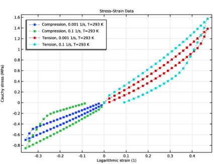
In the Settings window for Table Graph, type Compression, 0.001 1/s, T=293 K in the Label text field.
|
|
3
|
|
4
|
|
5
|
|
6
|
Locate the Coloring and Style section. Find the Line style subsection. From the Line list, choose Dotted.
|
|
7
|
|
8
|
|
9
|
|
10
|
Select the Label checkbox.
|
|
1
|
|
2
|
|
3
|
|
1
|
|
2
|
|
3
|
|
1
|
|
2
|
|
3
|
|
4
|
|
1
|
|
2
|
|
3
|
Locate the Parameters section. In the table, enter the following settings:
|
|
1
|
|
2
|
|
3
|
Locate the Parameters section. In the table, enter the following settings:
|
|
1
|
|
2
|
|
3
|
|
4
|
|
5
|
|
1
|
|
2
|
|
3
|
|
1
|
|
2
|
Select the object blk1 only.
|
|
3
|
|
4
|
|
5
|
|
6
|
|
7
|
|
1
|
In the Model Builder window, under Component 1 (comp1) right-click Materials and choose Blank Material.
|
|
2
|
|
3
|
Click to expand the Material Properties section. In the Material properties tree, select Solid Mechanics > Hyperelastic Material > Arruda–Boyce.
|
|
4
|
Click
|
|
5
|
In the Material properties tree, select Solid Mechanics > Viscoplastic Material > Bergstrom–Boyce Viscoplasticity.
|
|
6
|
Click
|
|
7
|
In the Model Builder window, expand the Component 1 (comp1) > Materials > Bergstrom–Boyce Material (mat1) node, then click Arruda–Boyce (ArrudaBoyce).
|
|
8
|
|
10
|
In the Model Builder window, under Component 1 (comp1) > Materials > Bergstrom–Boyce Material (mat1) click Bergstrom–Boyce viscoplasticity (BergstromBoyce).
|
|
11
|
|
1
|
|
2
|
|
3
|
From the list, choose Quasistatic.
|
|
4
|
|
1
|
|
2
|
Click in the Graphics window and then press Ctrl+A to select both domains.
|
|
3
|
|
4
|
|
5
|
|
6
|
|
7
|
|
1
|
|
2
|
|
3
|
|
4
|
|
5
|
|
6
|
|
7
|
|
8
|
Locate the Model Input section. From the T list, choose User defined. In the associated text field, type T.
|
|
1
|
|
1
|
|
2
|
In the Settings window for Prescribed Displacement, type Uniaxial Compression in the Label text field.
|
|
4
|
Locate the Prescribed Displacement section. From the Displacement in x direction list, choose Prescribed.
|
|
5
|
|
1
|
|
2
|
|
4
|
Locate the Prescribed Displacement section. In the u 0 x text field, type emax_ten*tri1(t/t_end)*1[mm].
|
|
1
|
|
1
|
|
2
|
|
3
|
|
4
|
|
1
|
|
2
|
|
3
|
|
4
|
|
1
|
|
1
|
|
1
|
|
2
|
In the Settings window for Variables, type Global Stress and Strain Variables in the Label text field.
|
|
3
|
Locate the Variables section. In the table, enter the following settings:
|
|
1
|
|
2
|
|
3
|
|
1
|
|
2
|
|
3
|
Click
|
|
1
|
|
2
|
|
3
|
|
1
|
|
2
|
|
3
|
In the Model Builder window, expand the Forward Problem > Solver Configurations > Solution 1 (sol1) > Dependent Variables 1 node, then click Viscoplastic Strain Tensor, Local Coordinate System (comp1.solid.hmm1.pvp1.evp).
|
|
4
|
|
5
|
|
6
|
In the Model Builder window, under Forward Problem > Solver Configurations > Solution 1 (sol1) > Dependent Variables 1 click Equivalent Viscoplastic Strain (comp1.solid.hmm1.pvp1.evpe).
|
|
7
|
|
8
|
|
9
|
In the Model Builder window, under Forward Problem > Solver Configurations > Solution 1 (sol1) > Dependent Variables 1 click Auxiliary Pressure (comp1.solid.hmm1.pw).
|
|
10
|
|
11
|
|
12
|
In the Model Builder window, under Forward Problem > Solver Configurations > Solution 1 (sol1) > Dependent Variables 1 click Displacement Field (comp1.u).
|
|
13
|
|
14
|
|
15
|
In the Model Builder window, under Forward Problem > Solver Configurations > Solution 1 (sol1) click Time-Dependent Solver 1.
|
|
16
|
|
17
|
|
18
|
Find the Algebraic variable settings subsection. From the Consistent initialization list, choose Off.
|
|
19
|
In the Model Builder window, under Forward Problem > Solver Configurations > Solution 1 (sol1) > Time-Dependent Solver 1 click Fully Coupled 1.
|
|
20
|
|
21
|
|
22
|
|
23
|
|
24
|
|
1
|
|
2
|
|
3
|
Locate the Data section. From the Dataset list, choose Forward Problem/Parametric Solutions 1 (sol2).
|
|
1
|
|
2
|
|
3
|
Locate the y-Axis Data section. In the table, enter the following settings:
|
|
4
|
|
5
|
|
6
|
|
7
|
|
1
|
|
2
|
|
3
|
Locate the y-Axis Data section. In the table, enter the following settings:
|
|
4
|
|
5
|
|
6
|
|
1
|
|
2
|
In the Settings window for Least-Squares Objective, type Compression, 0.001 1/s, T=293 K in the Label text field.
|
|
3
|
|
4
|
Locate the Data Column Settings section. In the table, enter the following settings:
|
|
6
|
|
7
|
|
8
|
|
9
|
|
1
|
|
2
|
In the Settings window for Least-Squares Objective, type Compression, 0.1 1/s, T=293 K in the Label text field.
|
|
3
|
Locate the Experimental Data section. From the Result table list, choose Compression, 0.1 1/s, T=293 K.
|
|
4
|
Locate the Data Column Settings section. In the table, click to select the cell at row number 3 and column number 1.
|
|
5
|
|
6
|
Locate the Experimental Conditions section. In the table, enter the following settings:
|
|
1
|
|
2
|
In the Settings window for Least-Squares Objective, type Tension, 0.001 1/s, T=293 K in the Label text field.
|
|
3
|
Locate the Experimental Data section. From the Result table list, choose Tension, 0.001 1/s, T=293 K.
|
|
4
|
Locate the Data Column Settings section. In the table, click to select the cell at row number 3 and column number 1.
|
|
5
|
|
6
|
|
7
|
Locate the Experimental Conditions section. In the table, enter the following settings:
|
|
1
|
|
2
|
In the Settings window for Least-Squares Objective, type Tension, 0.1 1/s, T=293 K in the Label text field.
|
|
3
|
|
4
|
Locate the Data Column Settings section. In the table, click to select the cell at row number 3 and column number 1.
|
|
5
|
|
6
|
Locate the Experimental Conditions section. In the table, enter the following settings:
|
|
1
|
|
2
|
Go to the Add Study window.
|
|
3
|
|
4
|
Click the Add Study button in the window toolbar.
|
|
5
|
|
1
|
|
2
|
|
1
|
|
2
|
|
3
|
|
4
|
Locate the Objective Function section. In the table, select the Active checkboxes for Compression, 0.001 1/s, T=293 K, Compression, 0.1 1/s, T=293 K, Tension, 0.001 1/s, T=293 K, and Tension, 0.1 1/s, T=293 K.
|
|
5
|
|
7
|
|
8
|
|
1
|
|
2
|
|
3
|
In the Model Builder window, expand the Parameter Estimation > Solver Configurations > Solution 5 (sol5) > Dependent Variables 1 node, then click Viscoplastic Strain Tensor, Local Coordinate System (comp1.solid.hmm1.pvp1.evp).
|
|
4
|
|
5
|
|
6
|
In the Model Builder window, under Parameter Estimation > Solver Configurations > Solution 5 (sol5) > Dependent Variables 1 click Equivalent Viscoplastic Strain (comp1.solid.hmm1.pvp1.evpe).
|
|
7
|
|
8
|
|
9
|
In the Model Builder window, under Parameter Estimation > Solver Configurations > Solution 5 (sol5) > Dependent Variables 1 click Auxiliary Pressure (comp1.solid.hmm1.pw).
|
|
10
|
|
11
|
|
12
|
In the Model Builder window, under Parameter Estimation > Solver Configurations > Solution 5 (sol5) > Dependent Variables 1 click Displacement Field (comp1.u).
|
|
13
|
|
14
|
|
15
|
In the Model Builder window, expand the Parameter Estimation > Solver Configurations > Solution 5 (sol5) > Optimization Solver 1 node, then click Time-Dependent Solver 1.
|
|
16
|
|
17
|
|
18
|
Find the Algebraic variable settings subsection. From the Consistent initialization list, choose Off.
|
|
19
|
In the Model Builder window, expand the Parameter Estimation > Solver Configurations > Solution 5 (sol5) > Optimization Solver 1 > Time-Dependent Solver 1 node, then click Fully Coupled 1.
|
|
20
|
|
21
|
|
22
|
|
23
|
|
1
|
|
2
|
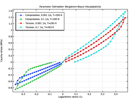
In the Settings window for 1D Plot Group, type Parameter Estimation: Bergstrom-Boyce Viscoplasticity in the Label text field.
|
|
3
|
|
1
|
|
2
|
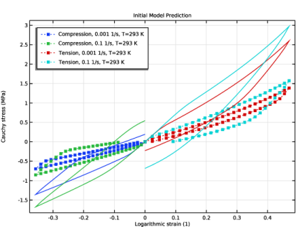
In the Settings window for Global, type Model Prediction, Compression 0.001 1/s in the Label text field.
|
|
3
|
Locate the y-Axis Data section. In the table, enter the following settings:
|
|
4
|
|
5
|
|
6
|
|
7
|
|
1
|
|
2
|
In the Settings window for Global, type Model Prediction, Compression 0.1 1/s in the Label text field.
|
|
3
|
Locate the y-Axis Data section. In the table, enter the following settings:
|
|
4
|
|
1
|
|
2
|
In the Settings window for Global, type Model Prediction, Tension 0.001 1/s in the Label text field.
|
|
3
|
Locate the y-Axis Data section. In the table, enter the following settings:
|
|
4
|
|
1
|
|
2
|
|
3
|
Locate the y-Axis Data section. In the table, enter the following settings:
|
|
1
|
|
2
|
|
3
|
Select the Plot checkbox.
|
|
5
|
Select the Show individual objective values checkbox.
|
|
6
|
Select the Table graph checkbox.
|
|
7
|
|
1
|
In the Model Builder window, under Component 1 (comp1) > Solid Mechanics (solid) right-click Hyperelastic Material 1 and choose Duplicate.
|
|
2
|
|
3
|
From the μ0 list, choose User defined. In the associated text field, type withsol('sol5', mu0_eq)*(1+(T-Tref)/Tref).
|
|
4
|
|
1
|
In the Model Builder window, expand the Hyperelastic Material 2 node, then click Polymer Viscoplasticity 1.
|
|
2
|
|
3
|
|
4
|
Find the Inelastic element subsection. From the A list, choose User defined. In the associated text field, type withsol('sol5', A).
|
|
5
|
|
6
|
|
7
|
From the σco list, choose User defined. Find the Isotropic hardening model subsection. From the c list, choose User defined. In the associated text field, type withsol('sol5', c).
|
|
1
|
|
2
|
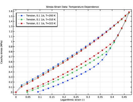
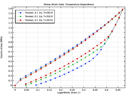
In the Settings window for 1D Plot Group, type Stress-Strain Data: Temperature Dependence in the Label text field.
|
|
3
|
|
4
|
|
5
|
|
1
|
|
2
|
|
3
|
|
4
|
|
5
|
|
6
|
|
7
|
Locate the Coloring and Style section. Find the Line style subsection. From the Line list, choose Dotted.
|
|
8
|
|
9
|
|
10
|
|
11
|
Clear the Headers checkbox.
|
|
12
|
|
1
|
|
2
|
|
3
|
|
1
|
|
2
|
|
3
|
|
4
|
|
1
|
|
2
|
In the Settings window for Least-Squares Objective, type Tension, 0.1 1/s, T=310 K in the Label text field.
|
|
3
|
|
4
|
Locate the Data Column Settings section. In the table, click to select the cell at row number 3 and column number 1.
|
|
5
|
|
6
|
|
1
|
|
2
|
In the Settings window for Least-Squares Objective, type Tension, 0.1 1/s, T=323 K in the Label text field.
|
|
3
|
|
4
|
Locate the Data Column Settings section. In the table, click to select the cell at row number 3 and column number 1.
|
|
5
|
|
6
|
Locate the Experimental Conditions section. In the table, enter the following settings:
|
|
1
|
|
2
|
Go to the Add Study window.
|
|
3
|
|
4
|
Click the Add Study button in the window toolbar.
|
|
5
|
|
1
|
In the Settings window for Study, type Parameter Estimation: Temperature Dependence in the Label text field.
|
|
2
|
|
1
|
|
2
|
|
3
|
|
4
|
Locate the Objective Function section. In the table, enter the following settings:
|
|
5
|
|
7
|
|
8
|
|
1
|
|
2
|
|
3
|
Select the Modify model configuration for study step checkbox.
|
|
4
|
In the tree, select Component 1 (comp1) > Solid Mechanics (solid), Controls spatial frame > Hyperelastic Material 1.
|
|
5
|
Click
|
|
1
|
|
2
|
Click
|
|
1
|
In the Model Builder window, right-click Stress–Strain Data: Temperature Dependence and choose Duplicate.
|
|
2
|
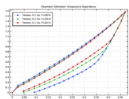
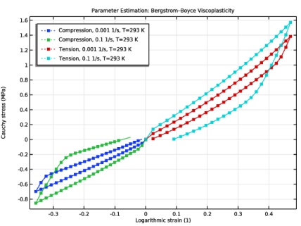
In the Settings window for 1D Plot Group, type Parameter Estimation: Temperature Dependence in the Label text field.
|
|
3
|
Locate the Data section. From the Dataset list, choose Parameter Estimation: Temperature Dependence/Solution 6 (sol6).
|
|
1
|
|
2
|
In the Settings window for Global, type Model Prediction, Tension 0.1 1/s, T=293 K in the Label text field.
|
|
3
|
Locate the Data section. From the Dataset list, choose Parameter Estimation: Temperature Dependence/Solution 6 (sol6).
|
|
4
|
|
5
|
|
6
|
Locate the y-Axis Data section. In the table, enter the following settings:
|
|
7
|
|
8
|
|
9
|
|
10
|
|
1
|
|
2
|
In the Settings window for Global, type Model Prediction, Tension 0.1 1/s, T=310 K in the Label text field.
|
|
3
|
|
4
|
Locate the y-Axis Data section. In the table, enter the following settings:
|
|
5
|
|
1
|
|
2
|
In the Settings window for Global, type Model Prediction, Tension 0.1 1/s, T=323 K in the Label text field.
|
|
3
|
|
4
|
Locate the y-Axis Data section. In the table, enter the following settings:
|
|
5
|
|
1
|
|
2
|
Go to the Result Templates window.
|
|
3
|
In the tree, select Parameter Estimation/Solution 5 (sol5) > Solid Mechanics > Estimated Parameters (std2).
|
|
4
|
Click the Add Result Template button in the window toolbar.
|
|
5
|
|
1
|
|
2
|
|
3
|
|
4
|
|
5
|
|
6
|
|
7
|
Locate the Expressions section. In the table, enter the following settings:
|
|
8
|