|
|
|
|
1
|
|
2
|
|
3
|
Click Add.
|
|
4
|
Click
|
|
5
|
|
6
|
Click
|
|
1
|
In the Model Builder window, click the root node.
|
|
2
|
|
3
|
From the Unit system list, choose MPa. The MPa base unit system is often convenient to use when working with structural mechanics problems.
|
|
1
|
|
2
|
|
3
|
|
4
|
|
5
|
Browse to the model’s Application Libraries folder and double-click the file parameter_estimation_plasticity_shear_data.txt.
|
|
1
|
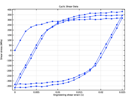
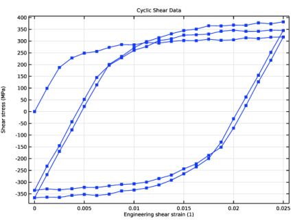
Go to the Cyclic Shear Data window.
|
|
2
|
Click the Table Graph button in the window toolbar.
|
|
1
|
|
2
|
|
3
|
|
4
|
|
5
|
Locate the Coloring and Style section. Find the Line markers subsection. From the Marker list, choose Point.
|
|
1
|
|
2
|
|
3
|
|
4
|
Locate the Plot Settings section.
|
|
5
|
|
6
|
|
7
|
|
1
|
|
2
|
|
3
|
|
4
|
Locate the Data Column Settings section. In the table, click to select the cell at row number 1 and column number 1.
|
|
5
|
|
7
|
|
8
|
|
9
|
Click
|
|
1
|
|
2
|
|
1
|
|
2
|
|
3
|
|
4
|
|
5
|
|
1
|
In the Model Builder window, under Component 1 (comp1) right-click Materials and choose Blank Material.
|
|
2
|
|
4
|
Click to expand the Material Properties section. In the Material properties tree, select Solid Mechanics > Elastoplastic Material > Elastoplastic Material Model.
|
|
5
|
Click
|
|
6
|
Locate the Material Contents section. In the table, enter the following settings:
|
|
7
|
Locate the Material Properties section. In the Material properties tree, select Solid Mechanics > Elastoplastic Material > Voce.
|
|
8
|
Click
|
|
9
|
Locate the Material Contents section. In the table, enter the following settings:
|
|
10
|
Locate the Material Properties section. In the Material properties tree, select Solid Mechanics > Elastoplastic Material > Armstrong–Frederick.
|
|
11
|
Click
|
|
12
|
Locate the Material Contents section. In the table, enter the following settings:
|
|
1
|
In the Model Builder window, expand the Material 1 (mat1) node, then click Component 1 (comp1) > Solid Mechanics (solid).
|
|
2
|
|
3
|
From the list, choose Quasistatic.
|
|
4
|
|
1
|
In the Model Builder window, under Component 1 (comp1) > Solid Mechanics (solid) click Linear Elastic Material 1.
|
|
2
|
|
3
|
|
4
|
|
1
|
|
2
|
|
3
|
Locate the Plasticity Model section. Find the Isotropic hardening model subsection. From the list, choose Voce.
|
|
4
|
|
1
|
|
1
|
|
1
|
|
3
|
|
4
|
|
5
|
|
6
|
|
7
|
|
1
|
|
1
|
|
2
|
|
1
|
|
1
|
|
2
|
|
3
|
|
4
|
|
1
|
|
2
|
|
3
|
|
4
|
|
1
|
|
2
|
|
3
|
Clear the Generate default plots checkbox.
|
|
4
|
|
1
|
|
2
|
|
3
|
Select the Auxiliary sweep checkbox.
|
|
4
|
Click
|
|
6
|
|
1
|
|
2
|
|
3
|
|
4
|
|
1
|
|
2
|
|
3
|
Select the Show legends checkbox.
|
|
4
|
|
1
|
|
2
|
|
4
|
|
5
|
|
6
|
|
7
|
|
1
|
|
2
|
|
3
|
|
4
|
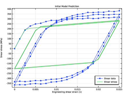
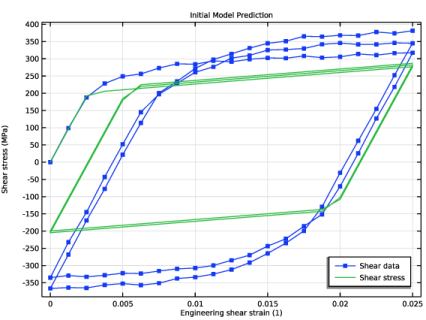
In the Initial Model Prediction toolbar, click
|
|
1
|
|
2
|
|
3
|
|
4
|
Locate the Data Column Settings section. In the table, enter the following settings:
|
|
5
|
|
6
|
|
9
|
|
10
|
|
11
|
|
1
|
|
2
|
Go to the Add Study window.
|
|
3
|
|
4
|
Click the Add Study button in the window toolbar.
|
|
5
|
|
1
|
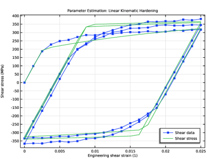
In the Settings window for Study, type Parameter Estimation: Linear Kinematic Hardening in the Label text field.
|
|
2
|
|
1
|
|
2
|
|
3
|
|
4
|
|
6
|
|
7
|
|
1
|
|
2
|
|
3
|
Select the Auxiliary sweep checkbox.
|
|
4
|
|
5
|
|
1
|
|
2
|
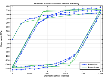
In the Settings window for 1D Plot Group, type Parameter Estimation: Linear Kinematic Hardening in the Label text field.
|
|
3
|
Locate the Data section. From the Dataset list, choose Parameter Estimation: Linear Kinematic Hardening/Solution 2 (sol2).
|
|
1
|
In the Model Builder window, under Parameter Estimation: Linear Kinematic Hardening click Parameter Estimation.
|
|
2
|
|
3
|
Select the Plot checkbox.
|
|
5
|
|
1
|
|
2
|
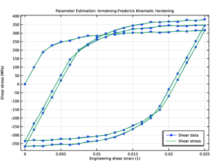
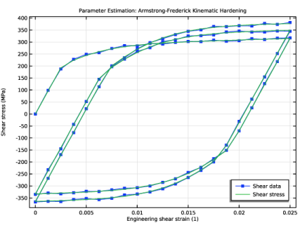
In the Settings window for Plasticity, type Armstrong-Frederick Kinematic Hardening in the Label text field.
|
|
3
|
Locate the Plasticity Model section. Find the Kinematic hardening model subsection. From the list, choose Armstrong–Frederick.
|
|
1
|
|
2
|
Go to the Add Study window.
|
|
3
|
|
4
|
Click the Add Study button in the window toolbar.
|
|
5
|
|
1
|
In the Settings window for Study, type Parameter Estimation: Armstrong-Frederick Kinematic Hardening in the Label text field.
|
|
2
|
|
1
|
|
2
|
|
3
|
|
4
|
|
6
|
|
7
|
|
1
|
|
2
|
|
3
|
Select the Auxiliary sweep checkbox.
|
|
4
|
|
5
|
|
1
|
In the Model Builder window, right-click Parameter Estimation: Linear Kinematic Hardening and choose Duplicate.
|
|
2
|
In the Settings window for 1D Plot Group, type Parameter Estimation: Armstrong-Frederick Kinematic Hardening in the Label text field.
|
|
3
|
Locate the Data section. From the Dataset list, choose Parameter Estimation: Armstrong-Frederick Kinematic Hardening/Solution 3 (sol3).
|
|
1
|
In the Model Builder window, under Parameter Estimation: Armstrong-Frederick Kinematic Hardening click Parameter Estimation.
|
|
2
|
|
3
|
Select the Plot checkbox.
|
|
5
|
|
1
|
|
2
|
Go to the Result Templates window.
|
|
3
|
In the tree, select Parameter Estimation: Linear Kinematic Hardening/Solution 2 (sol2) > Solid Mechanics > Estimated Parameters (std2).
|
|
4
|
Click the Add Result Template button in the window toolbar.
|
|
1
|
Go to the Result Templates window.
|
|
2
|
In the tree, select Parameter Estimation: Armstrong-Frederick Kinematic Hardening/Solution 3 (sol3) > Solid Mechanics > Estimated Parameters (std3).
|
|
3
|
Click the Add Result Template button in the window toolbar.
|
|
4
|
|
1
|
In the Settings window for Evaluation Group, type Estimated Parameters: Armstrong-Frederick Kinematic Hardening in the Label text field.
|