|
|
|


|
1
|
|
2
|
|
3
|
Click Add.
|
|
4
|
Click
|
|
5
|
|
6
|
Click
|
|
1
|
In the Model Builder window, click the root node.
|
|
2
|
|
3
|
From the Unit system list, choose MPa. The MPa base unit system is often convenient to use when working with structural mechanics problems.
|
|
1
|
|
2
|
|
3
|
|
4
|
|
5
|
Browse to the model’s Application Libraries folder and double-click the file parameter_estimation_hyperelasticity_uniaxial.txt.
|
|
1
|
|
2
|
|
3
|
|
4
|
Browse to the model’s Application Libraries folder and double-click the file parameter_estimation_hyperelasticity_pure_shear.txt.
|
|
1
|
|
2
|
|
3
|
|
4
|
Browse to the model’s Application Libraries folder and double-click the file parameter_estimation_hyperelasticity_equibiaxial.txt.
|
|
1
|
|
2
|
|
3
|
|
4
|
Locate the Plot Settings section.
|
|
5
|
|
6
|
|
7
|
|
1
|
|
2
|
|
3
|
Locate the Coloring and Style section. Find the Line style subsection. From the Line list, choose None.
|
|
4
|
|
5
|
|
6
|
|
7
|
|
1
|
|
2
|
|
3
|
|
4
|
|
5
|
Locate the Legends section. In the table, enter the following settings:
|
|
1
|
|
2
|
|
3
|
|
4
|
Locate the Legends section. In the table, enter the following settings:
|
|
5
|
|
1
|
|
2
|
|
1
|
|
2
|
|
3
|
|
1
|
|
2
|
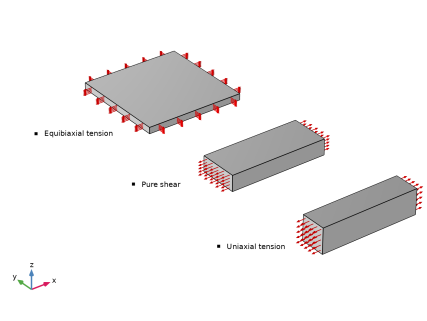
Select the object blk1 only.
|
|
3
|
|
4
|
|
5
|
|
6
|
|
7
|
|
1
|
|
2
|
|
3
|
From the list, choose Quasistatic.
|
|
4
|
|
1
|
|
2
|
Click in the Graphics window and then press Ctrl+A to select all domains.
|
|
3
|
|
4
|
|
5
|
|
6
|
Click
|
|
7
|
In the Ogden parameters table, enter the following settings:
|
|
8
|
|
1
|
|
1
|
|
3
|
|
4
|
|
5
|
|
1
|
|
3
|
|
4
|
|
1
|
|
3
|
|
4
|
|
5
|
|
1
|
|
1
|
|
2
|
|
3
|
|
4
|
|
1
|
|
2
|
|
3
|
|
4
|
|
1
|
|
2
|
|
4
|
|
5
|
|
1
|
|
1
|
|
1
|
|
2
|
|
1
|
|
2
|
|
3
|
|
1
|
|
2
|
|
3
|
Select the Auxiliary sweep checkbox.
|
|
4
|
Click
|
|
1
|
|
2
|
|
3
|
In the Model Builder window, expand the Forward Problem > Solver Configurations > Solution 1 (sol1) > Dependent Variables 1 node, then click Auxiliary Pressure (comp1.solid.hmm1.pw).
|
|
4
|
|
5
|
|
6
|
|
7
|
In the Model Builder window, under Forward Problem > Solver Configurations > Solution 1 (sol1) > Dependent Variables 1 click Displacement Field (comp1.u).
|
|
8
|
|
9
|
|
10
|
In the Model Builder window, expand the Forward Problem > Solver Configurations > Solution 1 (sol1) > Stationary Solver 1 node, then click Fully Coupled 1.
|
|
11
|
|
12
|
|
13
|
|
1
|
|
2
|
|
3
|
|
1
|
|
2
|
|
3
|
Locate the y-Axis Data section. In the table, enter the following settings:
|
|
4
|
|
5
|
|
6
|
|
8
|
|
1
|
|
2
|
In the Settings window for Least-Squares Objective, type Uniaxial Tension Test in the Label text field.
|
|
3
|
|
4
|
Locate the Data Column Settings section. In the table, enter the following settings:
|
|
5
|
|
6
|
|
8
|
|
9
|
|
10
|
|
1
|
|
2
|
|
3
|
|
4
|
|
5
|
Locate the Data Column Settings section. In the table, enter the following settings:
|
|
6
|
|
7
|
|
9
|
|
10
|
|
11
|
|
1
|
|
2
|
In the Settings window for Least-Squares Objective, type Equibiaxial Tension Test in the Label text field.
|
|
3
|
|
4
|
|
5
|
Locate the Data Column Settings section. In the table, enter the following settings:
|
|
6
|
|
7
|
|
9
|
|
10
|
|
11
|
|
1
|
|
2
|
Go to the Add Study window.
|
|
3
|
|
4
|
Click the Add Study button in the window toolbar.
|
|
5
|
|
1
|
|
2
|
|
1
|
|
2
|
|
3
|
|
4
|
|
6
|
|
7
|
|
1
|
|
2
|
|
3
|
Select the Auxiliary sweep checkbox.
|
|
4
|
|
5
|
|
1
|
|
2
|
|
3
|
In the Model Builder window, expand the Parameter Estimation > Solver Configurations > Solution 2 (sol2) > Dependent Variables 1 node, then click Auxiliary Pressure (comp1.solid.hmm1.pw).
|
|
4
|
|
5
|
|
6
|
|
7
|
In the Model Builder window, under Parameter Estimation > Solver Configurations > Solution 2 (sol2) > Dependent Variables 1 click Displacement Field (comp1.u).
|
|
8
|
|
9
|
|
10
|
In the Model Builder window, expand the Parameter Estimation > Solver Configurations > Solution 2 (sol2) > Optimization Solver 1 > Stationary Solver 1 node, then click Fully Coupled 1.
|
|
11
|
|
12
|
|
1
|
|
2
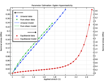
|
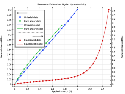
In the Settings window for 1D Plot Group, type Parameter Estimation: Ogden Hyperelasticity in the Label text field.
|
|
3
|
|
4
|
|
5
|
Locate the Plot Settings section.
|
|
6
|
|
7
|
|
8
|
Select the Two y-axes checkbox.
|
|
9
|
Select the Secondary y-axis label checkbox. In the associated text field, type Nominal stress (MPa).
|
|
10
|
|
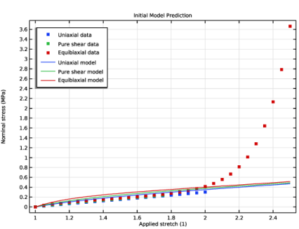
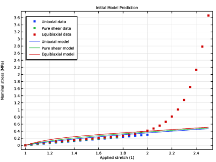
1
|
In the Model Builder window, under Results > Initial Model Prediction, Ctrl-click to select Uniaxial Data, Pure Shear Data, and Equibiaxial Data.
|
|
2
|
Right-click and choose Copy.
|
|
1
|
|
2
|
Select the Plot on secondary y-axis checkbox.
|
|
3
|
|
1
|
|
2
|
|
3
|
Locate the y-Axis Data section. In the table, enter the following settings:
|
|
4
|
|
5
|
|
1
|
|
2
|
|
3
|
Locate the y-Axis Data section. In the table, enter the following settings:
|
|
4
|
|
5
|
Locate the Legends section. In the table, enter the following settings:
|
|
1
|
|
2
|
|
3
|
|
4
|
Locate the y-Axis Data section. In the table, enter the following settings:
|
|
5
|
Locate the Legends section. In the table, enter the following settings:
|
|
1
|
|
2
|
|
3
|
|
1
|
|
2
|
|
3
|
|
1
|
|
2
|
|
3
|
Select the Plot checkbox.
|
|
5
|
Select the Show individual objective values checkbox.
|
|
6
|
Select the Table graph checkbox.
|
|
7
|
|
1
|
|
2
|
Go to the Result Templates window.
|
|
3
|
In the tree, select Parameter Estimation/Solution 2 (sol2) > Solid Mechanics > Estimated Parameters (std2).
|
|
4
|
Click the Add Result Template button in the window toolbar.
|
|
5
|