PDF

Hyperelastic Seal
Introduction
In this example you study the force–deflection relation of a car door seal made from a soft rubber material. The model uses a hyperelastic material together with formulations that can account for the large deformations and contact conditions. It is of special interest to investigate the effect of air confined within the seal.
See the Structural Mechanics Module User’s Guide for theory about hyperelastic material.
Model Definition
The seal is compressed between a stationary plane surface and an indenting cylinder. There is also a vertical rigid wall at a distance of 1 mm from the initial position of the seal. Figure 1 shows the undeformed geometry of the seal and the contacting surfaces.
Figure 1: Model geometry.
The seal is modeled in 2D assuming plane strain conditions. The (arbitrary) thickness in the out-of-plane direction is 50 mm. The contacting surfaces are rigid when compared to the seal.
Material Properties
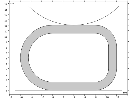
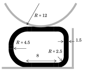
The rubber is hyperelastic and modeled as a Mooney-Rivlin material with C10 = 0.37 MPa and C01 = 0.11 MPa. The material is almost incompressible, so the bulk modulus is set to 104 MPa. A mixed formulation is automatically used for this material model.
Here, the undeformed and deformed cross-section areas are denoted by Aref and A, respectively. The ratio of specific heat, γ, has the value 1.4 and pref = 1 atm is the reference air pressure. The load acting on the interior of the seal is then
Constraints and Loads
Results and Discussion
Figure 2 shows the deformed shape at the lowest cylinder position — corresponding to an indentation of mm — without internal pressure. The deformation scale is 1:1, that is, a true shape. The plot shows a detachment region of significant size.
Figure 2: Seal deformation at 4 mm indentation without internal air pressure.
Figure 3 shows the corresponding contact pressure plot. The detachment region appears first at an indentation just over 2.5 mm and grows as the indentation increases further. The actual contact areas are reduced to two spots at the sides.
Such a significant change in the contact pressure distribution indicates that the computations must be performed using a fine mesh together with sufficiently small steps in the parametric analysis with respect to the indentation value.
Figure 3: The contact pressure distribution over the area between the seal and cylinder for different indentations without internal air pressure.
Figure 4 shows the result of the computations with the internal pressure taken into account. The seal profile appears inflated. The contact pressure plot in Figure 5 confirms that there is no detachment region even though the contact pressure has a pronounced minimum in the middle part.
Figure 4: Seal deformation at 4 mm indentation with internal air pressure.
Figure 5: The contact pressure distribution for different indentations with internal air pressure taken into account.
Figure 6 shows a plot of the force per unit length versus the indentation of the rigid cylinder, with and without the internal pressure taken into account. The distinct change in slope of the curves is attributed to the rightmost part of the seal coming into contact with the vertical wall, so that the seal can no longer deform in that direction.
Notice that the forces needed to compress the seal can be almost one order of magnitude larger when the effect of the confined air is taken into account.
In reality, a car door seal contains small holes through which the air can escape as long as the compression is not too fast. Thus, the values computed with and without internal air pressure are the limits corresponding to very fast and very slow compression, respectively.
Figure 6: Compressive force per unit length versus indentation with and without internal pressure.
Notes About the COMSOL Implementation
The confined air inside the seal is modeled using an Enclosed Cavity node, which automatically computes the undeformed and deformed volume (or cross-section area) enclosed by the inner seal boundaries with the divergence theorem. The Fluid subnode adds the pressure load resulting from the volume change, in this case assuming the adiabatic compression of air.
Application Library path: Nonlinear_Structural_Materials_Module/Hyperelasticity/hyperelastic_seal
Modeling Instructions
From the File menu, choose New.
New
In the New window, click  Model Wizard.
Model Wizard
1
In the Model Wizard window, click  2D.
2
In the Select Physics tree, select Structural Mechanics > Solid Mechanics (solid).
3
Click Add.
4
Click  Study.
5
In the Select Study tree, select General Studies > Stationary.
6
Geometry 1
If you do not want to build all the geometry, you can load the geometry sequence from the stored model. In the Model Builder window, under Component 1 (comp1) right-click Geometry 1 and choose Insert Sequence. Browse to the model’s Application Libraries folder and double-click the file hyperelastic_seal.mph. You can then continue to the Global Definitions section below.
To build the geometry from scratch, continue from here.
1
In the Model Builder window, under Component 1 (comp1) click Geometry 1.
2
In the Settings window for Geometry, locate the Units section.
3
From the Length unit list, choose mm.
Rectangle 1 (r1)
1
In the Geometry toolbar, click  Rectangle.
2
In the Settings window for Rectangle, locate the Object Type section.
3
From the Type list, choose Curve.
4
Locate the Size and Shape section. In the Width text field, type 18.
5
In the Height text field, type 12.
6
Locate the Position section. In the x text field, type -6.
7
Click  Build Selected.
Fillet 1 (fil1)
1
In the Geometry toolbar, click  Fillet.
2
On the object r1, select Points 1 and 4 only.
3
In the Settings window for Fillet, locate the Radius section.
4
In the Radius text field, type 6.
5
Click  Build Selected.
Fillet 2 (fil2)
1
In the Geometry toolbar, click  Fillet.
2
On the object fil1, select Points 4 and 5 only.
3
In the Settings window for Fillet, locate the Radius section.
4
In the Radius text field, type 4.
5
Click  Build Selected.
Thicken 1 (thi1)
1
In the Geometry toolbar, click  Conversions and choose Thicken.
2
3
In the Settings window for Thicken, locate the Options section.
4
From the Offset list, choose Asymmetric.
5
In the Upside thickness text field, type 1.5.
6
Click  Build Selected.
Create the indenter.
Indenter
1
In the Geometry toolbar, click  Circle.
2
In the Settings window for Circle, type Indenter in the Label text field.
3
Locate the Size and Shape section. In the Radius text field, type 12.
4
In the Sector angle text field, type 90.
5
Locate the Position section. In the x text field, type 4.
6
In the y text field, type 24.
7
Locate the Rotation Angle section. In the Rotation text field, type -135.
8
Locate the Selections of Resulting Entities section. Select the Resulting objects selection checkbox.
9
From the Show in physics list, choose Boundary selection.
Create the support.
Rectangle 2 (r2)
1
In the Geometry toolbar, click  Rectangle.
2
In the Settings window for Rectangle, locate the Size and Shape section.
3
In the Width text field, type 20.
4
Locate the Position section. In the x text field, type -7.
5
In the y text field, type -1.
6
Locate the Selections of Resulting Entities section. Select the Resulting objects selection checkbox.
7
From the Show in physics list, choose Boundary selection.
8
Find the Cumulative selection subsection. Click New.
9
In the New Cumulative Selection dialog, type Rigid base in the Name text field.
10
Rectangle 3 (r3)
1
In the Geometry toolbar, click  Rectangle.
2
In the Settings window for Rectangle, locate the Size and Shape section.
3
In the Height text field, type 12.
4
Locate the Position section. In the x text field, type 13.
5
Locate the Selections of Resulting Entities section. Find the Cumulative selection subsection. From the Contribute to list, choose Rigid base.
Convert to Curve 1 (ccur1)
1
In the Geometry toolbar, click  Conversions and choose Convert to Curve.
2
Select the objects c1, r2, and r3 only.
3
In the Settings window for Convert to Curve, click  Build Selected.
Delete Entities 1 (del1)
1
In the Model Builder window, right-click Geometry 1 and choose Delete Entities.
2
On the object ccur1, select Boundaries 1, 2, 4–6, and 8–10 only.
Form Union (fin)
1
In the Model Builder window, under Component 1 (comp1) > Geometry 1 click Form Union (fin).
2
In the Settings window for Form Union/Assembly, locate the Form Union/Assembly section.
3
From the Action list, choose Form an assembly.
4
Clear the Create pairs checkbox.
5
Click  Build Selected.
6
Click the  Zoom Extents button in the Graphics toolbar.
The model geometry is now complete.
Inner Seal Boundary
1
In the Geometry toolbar, click  Selections and choose Explicit Selection.
2
In the Settings window for Explicit Selection, type Inner Seal Boundary in the Label text field.
3
Locate the Entities to Select section. From the Geometric entity level list, choose Boundary.
4
Select the Group by continuous tangent checkbox.
5
Outer Seal Boundary
1
In the Geometry toolbar, click  Selections and choose Explicit Selection.
2
In the Settings window for Explicit Selection, type Outer Seal Boundary in the Label text field.
3
Locate the Entities to Select section. From the Geometric entity level list, choose Boundary.
4
Select the Group by continuous tangent checkbox.
5
Glued Seal Boundary
1
In the Geometry toolbar, click  Selections and choose Explicit Selection.
2
In the Settings window for Explicit Selection, type Glued Seal Boundary in the Label text field.
3
Locate the Entities to Select section. From the Geometric entity level list, choose Boundary.
4
On the object fin, select Boundary 4 only.
Fillet 1 (fil1), Fillet 2 (fil2), Rectangle 1 (r1), Thicken 1 (thi1)
1
In the Model Builder window, under Component 1 (comp1) > Geometry 1, Ctrl-click to select Rectangle 1 (r1), Fillet 1 (fil1), Fillet 2 (fil2), and Thicken 1 (thi1).
2
Seal
In the Settings window for Group, type Seal in the Label text field.
Global Definitions
Add a parameter that you can use to gradually increase the vertical displacement.
Parameters 1
1
In the Model Builder window, under Global Definitions click Parameters 1.
2
In the Settings window for Parameters, locate the Parameters section.
3
Definitions
Contact Pair 1 (p1)
1
In the Definitions toolbar, click  Pairs and choose Contact Pair.
2
In the Settings window for Pair, type upper in the Pair name text field.
3
Locate the Source Boundaries section. From the Selection list, choose Indenter.
4
Locate the Destination Boundaries section. From the Selection list, choose Outer Seal Boundary.
Contact Pair 2 (p2)
1
In the Definitions toolbar, click  Pairs and choose Contact Pair.
2
In the Settings window for Pair, type lower in the Pair name text field.
3
Locate the Source Boundaries section. From the Selection list, choose Rigid base.
4
Locate the Destination Boundaries section. From the Selection list, choose Outer Seal Boundary.
The boundaries in the contact pairs are unnecessarily large because it was convenient to reuse existing selections. In large 3D models, you should however keep down the size of the contact boundaries for performance reasons.
Since the indenter is only modeled as a rigid boundary, prescribe its deformation using a moving mesh. Alternatively, the indenter could be modeled as a rigid or elastic domain in the Solid Mechanics interface, in which case its deformation would be prescribed in the interface.
Component 1 (comp1)
Prescribed Deformation 1
1
In the Physics toolbar, click  Moving Mesh and choose Prescribed Deformation.
2
In the Settings window for Prescribed Deformation, locate the Geometric Entity Selection section.
3
From the Geometric entity level list, choose Boundary.
4
From the Selection list, choose Indenter.
5
Locate the Prescribed Deformation section. Specify the dx vector as
Solid Mechanics (solid)
1
In the Model Builder window, under Component 1 (comp1) click Solid Mechanics (solid).
2
In the Settings window for Solid Mechanics, locate the Thickness section.
3
In the d text field, type d. In the plane strain approximation, this setting only affects total force computations.
Hyperelastic Material 1
1
In the Physics toolbar, click  Domains and choose Hyperelastic Material.
2
In the Settings window for Hyperelastic Material, locate the Domain Selection section.
3
From the Selection list, choose All domains.
4
Locate the Hyperelastic Material section. From the Material model list, choose Mooney–Rivlin, two parameters.
5
In the κ text field, type 1e4[MPa].
Contact 1
In the Model Builder window, click Contact 1.
Friction 1
1
In the Physics toolbar, click  Attributes and choose Friction.
2
In the Settings window for Friction, locate the Friction Parameters section.
3
In the μ text field, type 0.3.
Add an adhesion condition to model the glue layer at the bottom of the seal.
Contact 1
In the Model Builder window, click Contact 1.
Adhesion 1
1
In the Physics toolbar, click  Attributes and choose Adhesion.
2
In the Settings window for Adhesion, locate the Adhesive Activation section.
3
From the Activation criterion list, choose User defined.
4
5
Locate the Adhesive Stiffness section. From the Adhesive stiffness list, choose User defined.
6
Specify the k vector as
Add an Enclosed Cavity node to model the effect of air being compressed inside the seal.
Enclosed Cavity 1
1
In the Physics toolbar, click  Boundaries and choose Enclosed Cavity.
2
In the Settings window for Enclosed Cavity, locate the Boundary Selection section.
3
From the Selection list, choose Inner Seal Boundary.
Fluid 1
Inspect the Fluid subnode, which defines the properties of the gas being compressed. To study the effect of the confined air, add the Fluid node to a load group.
1
In the Model Builder window, click Fluid 1.
2
In the Physics toolbar, click  Load Group and choose New Load Group.
Materials
Material 1 (mat1)
1
In the Model Builder window, under Component 1 (comp1) right-click Materials and choose Blank Material.
2
In the Settings window for Material, locate the Material Contents section.
3
Mesh 1
Edge 1
1
In the Mesh toolbar, click  More Generators and choose Edge.
2
Distribution 1
1
Right-click Edge 1 and choose Distribution.
2
In the Settings window for Distribution, locate the Distribution section.
3
In the Number of elements text field, type 1.
4
Locate the Boundary Selection section. From the Selection list, choose Rigid base.
Distribution 2
1
In the Model Builder window, right-click Edge 1 and choose Distribution.
2
In the Settings window for Distribution, locate the Distribution section.
3
In the Number of elements text field, type 50.
4
Locate the Boundary Selection section. From the Selection list, choose Indenter.
Free Quad 1
In the Mesh toolbar, click  Free Quad.
Size 1
1
Right-click Free Quad 1 and choose Size.
2
In the Settings window for Size, locate the Geometric Entity Selection section.
3
From the Geometric entity level list, choose Boundary.
4
From the Selection list, choose Inner Seal Boundary.
5
Locate the Element Size section. Click the Custom button.
6
Locate the Element Size Parameters section.
7
Select the Maximum element size checkbox. In the associated text field, type 0.2.
Size 2
1
Right-click Size 1 and choose Duplicate.
2
In the Settings window for Size, locate the Geometric Entity Selection section.
3
From the Selection list, choose Outer Seal Boundary.
4
Click  Build All.
Study 1
Step 1: Stationary
Set up an auxiliary continuation sweep for the parameter para. Start at a nonzero value to avoid ill-conditioning during contact initiation.
1
In the Model Builder window, under Study 1 click Step 1: Stationary.
2
In the Settings window for Stationary, click to expand the Study Extensions section.
3
Select the Auxiliary sweep checkbox.
4
5
Define two load cases to study the effect of the confined air.
6
Select the Define load cases checkbox.
7
8
9
10
In the Study toolbar, click  Get Initial Value.
Set default units for result presentation.
Results
Preferred Units 1
1
In the Results toolbar, click  Configurations and choose Preferred Units.
2
In the Settings window for Preferred Units, locate the Units section.
3
Click  Add Physical Quantity.
4
In the Physical Quantity dialog, select Solid Mechanics > Stress tensor (N/m^2) in the tree.
5
6
In the Settings window for Preferred Units, locate the Units section.
7
8
Click  Add Physical Quantity.
9
In the Physical Quantity dialog, select Solid Mechanics > Face load (N/m^2) in the tree.
10
11
In the Settings window for Preferred Units, locate the Units section.
12
13
Click  Apply.
Stress (solid)
Add an Arrow Line plot to visualize the gas pressure.
Arrow Line 1
1
In the Model Builder window, right-click Stress (solid) and choose Arrow Line.
2
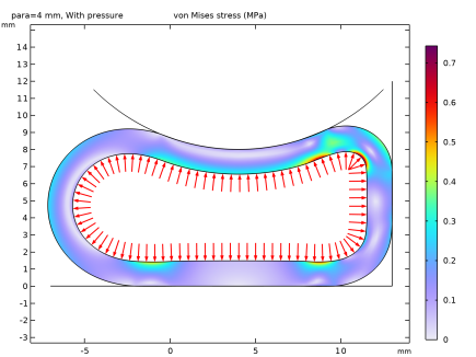
In the Settings window for Arrow Line, click Replace Expression in the upper-right corner of the Expression section. From the menu, choose Component 1 (comp1) > Solid Mechanics > Enclosed cavities > Enclosed Cavity 1 > solid.enc1.fax,solid.enc1.fay - Force per deformed area (spatial frame).
3
Click to expand the Title section. From the Title type list, choose None.
4
Locate the Arrow Positioning section. In the Number of arrows text field, type 300.
5
Locate the Coloring and Style section. From the Arrow base list, choose Head.
6
Click to expand the Inherit Style section. From the Plot list, choose Surface 1.
7
Clear the Color checkbox.
8
Clear the Color and data range checkbox.
Study 1
Solver Configurations
In the Model Builder window, expand the Study 1 > Solver Configurations node.
Solution 1 (sol1)
1
In the Model Builder window, expand the Study 1 > Solver Configurations > Solution 1 (sol1) node.
The default scale for the displacement variables is calculated from the entire geometry size. For models with prescribed displacements as domain or boundary constraints, the maximum prescribed displacement usually gives a better estimate of the scale.
2
In the Model Builder window, expand the Study 1 > Solver Configurations > Solution 1 (sol1) > Dependent Variables 1 node, then click Displacement Field (comp1.u).
3
In the Settings window for Field, locate the Scaling section.
4
In the Scale text field, type 1e-3.
Change the scale for the auxiliary pressure to account for the material properties of the seal made of soft rubber.
5
In the Model Builder window, click Auxiliary Pressure (comp1.solid.hmm1.pw).
6
In the Settings window for Field, locate the Scaling section.
7
In the Scale text field, type 1e5.
8
In the Model Builder window, expand the Study 1 > Solver Configurations > Solution 1 (sol1) > Stationary Solver 1 node, then click Direct.
9
In the Settings window for Direct, locate the General section.
10
From the Solver list, choose PARDISO.
Step 1: Stationary
1
In the Model Builder window, under Study 1 click Step 1: Stationary.
2
In the Settings window for Stationary, click to expand the Results While Solving section.
3
Select the Plot checkbox.
4
In the Study toolbar, click  Compute.
Results
Stress (solid)
1
Click the  Zoom Extents button in the Graphics toolbar.
2
In the Settings window for 2D Plot Group, clicknext to  cycle_plot_level, then choose Load case.
3
Click  Plot First.
4
Click the  Zoom Extents button in the Graphics toolbar.
The default plot shows the von Mises stress distribution in the seal. The case without confined air is shown in Figure 2.
Next, visualize the stress distribution with confined air.
5
Click  Plot Last.
You can see that the detachment region has disappeared as a result of the seal pressurization, compare with Figure 4.
Add a plot from Result Templates to visualize the normal and tangential contact forces on the seal.
Result Templates
1
In the Results toolbar, click  Result Templates to open the Result Templates window.
2
Go to the Result Templates window.
3
In the tree, select Study 1/Solution 1 (sol1) > Solid Mechanics > Contact Forces (solid).
4
Click the Add Result Template button in the window toolbar.
5
In the Results toolbar, click  Result Templates to close the Result Templates window.
Results
Contact Forces (solid)
In the Model Builder window, expand the Results > Contact Forces (solid) node.
Color Expression
1
In the Model Builder window, expand the Results > Contact Forces (solid) > Contact 1, Pressure node, then click Color Expression.
2
In the Settings window for Color Expression, locate the Expression section.
3
From the Unit list, choose kPa.
Color Expression
1
In the Model Builder window, expand the Results > Contact Forces (solid) > Contact 1, Friction Force node, then click Color Expression.
2
In the Settings window for Color Expression, locate the Expression section.
3
From the Unit list, choose kPa.
The following steps show how to display the contact pressure at the bottom of the seal.
Contact Pressure
1
In the Results toolbar, click  1D Plot Group.
2
In the Settings window for 1D Plot Group, type Contact Pressure in the Label text field.
3
Locate the Data section. From the Parameter selection (Load case) list, choose First.
4
From the Parameter selection (para) list, choose Manual.
5
In the Parameter indices (1-41) text field, type range(10,5,40).
6
Click to expand the Title section. From the Title type list, choose Manual.
7
In the Title text area, type Contact pressure profile.
Line Graph 1
1
Right-click Contact Pressure and choose Line Graph.
2
3
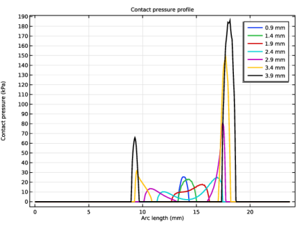
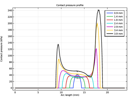
In the Settings window for Line Graph, click Replace Expression in the upper-right corner of the y-Axis Data section. From the menu, choose Component 1 (comp1) > Solid Mechanics > Contact > solid.Tn - Contact pressure - N/m².
4
Click to expand the Legends section. Select the Show legends checkbox.
5
Find the Include subsection. Clear the Solution checkbox.
6
Find the Prefix and suffix subsection. In the Prefix text field, type eval(para) mm.
7
Click to expand the Coloring and Style section. From the Width list, choose 2.
8
In the Contact Pressure toolbar, click  Plot.
The plot in the Graphics window should now look like that in Figure 3.
Contact Pressure
Next, plot the pressure profile when the internal air pressure is included.
1
In the Model Builder window, click Contact Pressure.
2
In the Settings window for 1D Plot Group, locate the Data section.
3
From the Parameter selection (Load case) list, choose Last.
4
In the Contact Pressure toolbar, click  Plot.
Finally, compute the force needed for the compression as the sum of all vertical reaction forces on the indenter.
Compressive Force vs. Indentation
1
In the Results toolbar, click  1D Plot Group.
2
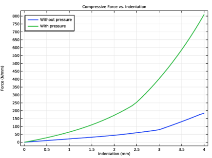
In the Settings window for 1D Plot Group, type Compressive Force vs. Indentation in the Label text field.
3
Locate the Title section. From the Title type list, choose Label.
Global 1
1
In the Compressive Force vs. Indentation toolbar, click  Global.
2
In the Settings window for Global, locate the y-Axis Data section.
3
4
Click to expand the Coloring and Style section. From the Width list, choose 2.
Compressive Force vs. Indentation
1
In the Model Builder window, click Compressive Force vs. Indentation.
2
In the Settings window for 1D Plot Group, locate the Plot Settings section.
3
Select the x-axis label checkbox.
4
Select the y-axis label checkbox.
5
In the x-axis label text field, type Indentation (mm).
6
In the y-axis label text field, type Force (N/mm).
7
Locate the Legend section. From the Position list, choose Upper left.
Compare with the plot shown in Figure 6.