PDF

Elastoplastic Analysis of Holed Plate
Introduction
In this example you analyze a perforated plate loaded into the plastic regime. In addition to the original problem, which you can find in section 7.10 of The Finite Element Method by O.C. Zienkiewicz (Ref. 1), you can also study the unloading of the plate.
The model also shows how to apply a user defined yield criterion and an external hardening function based on an interpolated stress–strain curve.
Model Definition
Figure 1 shows the plate’s geometry. Due to the double symmetry of the geometry you only need to analyze a quarter of the plate.
Figure 1: The plate geometry.
Because the plate is thin and the loads are in plane, you can assume a plane stress condition.
Material
Elastic properties: E = 70000 MPa and ν = 0.2.
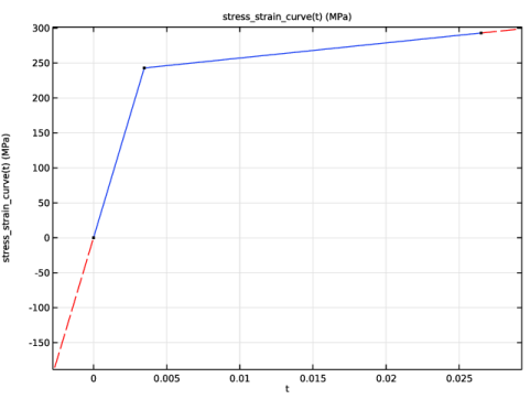
Plastic properties: Yield stress 243 MPa and a linear isotropic hardening with tangent modulus 2171 MPa.
Constraints and loads
The right vertical edge is subjected to a stress, which increases from zero to a maximum value of 133.65 MPa and then is released again. The peak value is selected so that the mean stress over the section through the hole is 10% above the yield stress (=1.1·243·(2010)/20).
Results and Discussion
Figure 2 shows the development of the plastic region. The parameter values are 0.55, 0.65, 0.75, 0.85, 0.95, and 1.05. These values are proportional to the load with a parameter value 1.0, which corresponds to the yield limit of the average stress over the cross section through the hole. For a material without strain hardening, the structure would thus have collapsed before reaching the final load level. Because an elastoplastic solution is load-path dependent, it is important not to use too large steps in the load parameter when you anticipate a plastic flow. Usually you can take one large step up to the elastic limit, as this example shows. Moreover, reversed plastic flow can occur during the unloading. This is why this study uses small parameter steps at the end of the parameter range.
Figure 2: Development of plastic region (blue) for parameter values 0.55, 0.65, 0.75, 0.85, 0.95 and 1.05.
Modeling with COMSOL Multiphysics
In this example there are two studies where the only difference is how the hardening data of the plasticity model is entered. In the first study, you give the data in the most natural way, since a linear hardening can be entered directly using the tangent modulus.
In the second study, it is shown how to proceed when you have a tabulated data from a general tensile test. Note that in metal plasticity, the hardening function σh to be entered is the stress added to the initial yield stress σys0 as function of the equivalent plastic strain εpe. Thus, the function must always pass the point (0,0). If your tabulated data contains total stress versus total strain, the hardening function must thus be written as
where, σe is the equivalent (von Mises) stress, E is the Young’s modulus, and σtab is an interpolation function of your tabulated data. Figure 4 shows the linear elastic and plastic regions.
Figure 3: The interpolated stress–strain curve shows both the elastic and hardening regions.
The results show in Figure 4 and Figure 5 are in good agreement. In Study 1, isotropic hardening is generated with an isotropic tangent modulus ETiso = 2.171 GPa, and in Study 2 it is generated with interpolated hardening function data, which mimics the isotropic tangent modulus from Study 1.
Figure 4: Deformation and von Mises stress for parameter value 2.2. The hardening was implemented with isotropic tangent modulus ETiso = 2.171 GPa.
Figure 5: Deformation and von Mises stress for parameter value 2.2. The hardening was implemented with the interpolated hardening function.
Reference
1. O.C. Zienkiewicz and R.L. Taylor, The Finite Element Method, 4th ed., McGraw Hill, 1991.
Application Library path: Nonlinear_Structural_Materials_Module/Plasticity/elastoplastic_plate
Modeling Instructions
From the File menu, choose New.
New
In the New window, click  Model Wizard.
Model Wizard
1
In the Model Wizard window, click  2D.
2
In the Select Physics tree, select Structural Mechanics > Solid Mechanics (solid).
3
Click Add.
4
Click  Study.
5
In the Select Study tree, select General Studies > Stationary.
6
Geometry 1
Begin by changing the length unit to millimeters.
1
In the Model Builder window, under Component 1 (comp1) click Geometry 1.
2
In the Settings window for Geometry, locate the Units section.
3
From the Length unit list, choose mm.
Rectangle 1 (r1)
1
In the Geometry toolbar, click  Rectangle.
2
In the Settings window for Rectangle, locate the Size and Shape section.
3
In the Width text field, type 18.
4
In the Height text field, type 10.
5
Click  Build Selected.
Circle 1 (c1)
1
In the Geometry toolbar, click  Circle.
2
In the Settings window for Circle, locate the Size and Shape section.
3
In the Radius text field, type 5.
4
Click  Build Selected.
Difference 1 (dif1)
1
In the Geometry toolbar, click  Booleans and Partitions and choose Difference.
2
3
In the Settings window for Difference, locate the Difference section.
4
Click to select the  Activate Selection toggle button for Objects to subtract.
5
6
Click  Build Selected.
Add a parameter for controlling the applied load.
Global Definitions
Parameters 1
1
In the Model Builder window, under Global Definitions click Parameters 1.
2
In the Settings window for Parameters, locate the Parameters section.
3
Definitions
Interpolation 1 (int1)
1
In the Definitions toolbar, click  Interpolation.
2
In the Settings window for Interpolation, locate the Definition section.
3
In the Function name text field, type loadfunc.
4
5
Locate the Units section. In the Argument table, enter the following settings:
6
In the Function table, enter the following settings:
7
An interpolation function is used to define the applied load.
Solid Mechanics (solid)
1
In the Model Builder window, under Component 1 (comp1) click Solid Mechanics (solid).
2
In the Settings window for Solid Mechanics, locate the 2D Approximation section.
3
4
Locate the Thickness section. In the d text field, type 10[mm].
Linear Elastic Material 1
In the Model Builder window, under Component 1 (comp1) > Solid Mechanics (solid) click Linear Elastic Material 1.
Linear Hardening
1
In the Physics toolbar, click  Attributes and choose Plasticity.
2
In the Settings window for Plasticity, type Linear Hardening in the Label text field.
Materials
Material 1 (mat1)
1
In the Model Builder window, under Component 1 (comp1) right-click Materials and choose Blank Material.
2
In the Settings window for Material, locate the Material Contents section.
3
Solid Mechanics (solid)
Symmetry 1
1
In the Physics toolbar, click  Boundaries and choose Symmetry.
2
Boundary Load 1
1
In the Physics toolbar, click  Boundaries and choose Boundary Load.
2
3
In the Settings window for Boundary Load, locate the Force section.
4
Specify the fA vector as
Mesh 1
Free Triangular 1
1
In the Mesh toolbar, click  Free Triangular.
The mesh should be refined in areas where large stress and strain gradients are anticipated.
Refine 1
1
In the Mesh toolbar, click  Modify and choose Refine.
2
In the Settings window for Refine, click to expand the Refine Elements in Box section.
3
Select the Specify bounding box checkbox.
4
In row x, set Upper bound to 8.
5
In row y, set Upper bound to 10.
6
In the Model Builder window, right-click Mesh 1 and choose Build All.
The mesh should consist of around 700 elements.
Study 1
Step 1: Stationary
Set up an auxiliary continuation sweep for the para parameter.
1
In the Model Builder window, under Study 1 click Step 1: Stationary.
2
In the Settings window for Stationary, click to expand the Study Extensions section.
3
Select the Auxiliary sweep checkbox.
4
5
With these settings, the boundary load you defined earlier increases from zero to a maximum value of 133.65 MPa and is then released.
6
In the Model Builder window, click Study 1.
7
In the Settings window for Study, type Linear Hardening in the Label text field.
8
Locate the Study Settings section. Clear the Generate default plots checkbox.
9
In the Study toolbar, click  Compute.
Add a plot of the von Mises stress in the plate at the final load increment from Result Templates.
Result Templates
1
In the Results toolbar, click  Result Templates to open the Result Templates window.
2
Go to the Result Templates window.
3
In the tree, select Linear Hardening/Solution 1 (sol1) > Solid Mechanics > Stress (solid).
4
Click the Add Result Template button in the window toolbar.
5
In the Results toolbar, click  Result Templates to close the Result Templates window.
Results
Stress, Linear Hardening
1
In the Settings window for 2D Plot Group, type Stress, Linear Hardening in the Label text field.
2
Click the  Zoom Extents button in the Graphics toolbar.
Visualize the plastic zone using the boolean expression solid.epeGp>0, which is 1 in the plastic region and 0 elsewhere.
Result Templates
1
In the Results toolbar, click  Result Templates to open the Result Templates window.
2
Go to the Result Templates window.
3
In the tree, select Linear Hardening/Solution 1 (sol1) > Solid Mechanics > Equivalent Plastic Strain (solid).
4
Click the Add Result Template button in the window toolbar.
5
In the Results toolbar, click  Result Templates to close the Result Templates window.
Results
Plastic Region, Linear Hardening
In the Settings window for 2D Plot Group, type Plastic Region, Linear Hardening in the Label text field.
Surface 1
1
In the Model Builder window, expand the Plastic Region, Linear Hardening node, then click Surface 1.
2
In the Settings window for Surface, locate the Expression section.
3
In the Expression text field, type solid.epeGp>0.
4
In the Plastic Region, Linear Hardening toolbar, click  Plot.
Plastic Region, Linear Hardening
1
Click the  Zoom Extents button in the Graphics toolbar.
2
In the Model Builder window, click Plastic Region, Linear Hardening.
3
In the Settings window for 2D Plot Group, locate the Data section.
4
From the Parameter value (para) list, choose 0.55.
5
In the Plastic Region, Linear Hardening toolbar, click  Plot.
The plot in the Graphics window should now look like that in the upper-left panel of Figure 2.
6
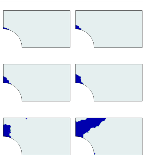
Repeat steps 3, 4 and 5 for Parameter value (para) 0.65, 0.75, 0.85, 0.95, and 1.05 to reproduce the remaining subplots in Figure 2.
Hardening with Experimental Stress–Strain Data and User-Defined Yield Function.
To fit the first study case, the stress–strain curve will be very simple, an elastic slope of 70 GPa and then a plastic slope of 2.171 GPa. Only three points are needed to define the stress–strain curve in this simple case.
Definitions
Interpolation 2 (int2)
1
In the Definitions toolbar, click  Interpolation.
2
In the Settings window for Interpolation, locate the Definition section.
3
In the Function name text field, type stress_strain_curve.
4
5
Locate the Units section. In the Argument table, enter the following settings:
6
In the Function table, enter the following settings:
7
Locate the Interpolation and Extrapolation section. From the Extrapolation list, choose Linear.
8
Add a variable for controlling the hardening.
Variables 1
1
In the Definitions toolbar, click  Local Variables.
2
In the Settings window for Variables, locate the Variables section.
3
Solid Mechanics (solid)
Linear Elastic Material 1
In the Model Builder window, under Component 1 (comp1) > Solid Mechanics (solid) click Linear Elastic Material 1.
Interpolated Hardening and User-Defined Plastic Flow
1
In the Physics toolbar, click  Attributes and choose Plasticity.
2
In the Settings window for Plasticity, type Interpolated Hardening and User-Defined Plastic Flow in the Label text field.
Define the von Mises stress in terms of the second invariant of the stress tensor.
3
Locate the Plasticity Model section. From the σe list, choose User defined.
4
In the text field, type sqrt(3*solid.II2sEff).
Add a small value to the potential to avoid possible division by zero when evaluating its derivative at zero stress.
5
From the Qp list, choose User defined.
6
In the text field, type sqrt(3*solid.II2sEff+eps).
7
Find the Isotropic hardening model subsection. From the list, choose Hardening function.
Materials
Material 1 (mat1)
Use hardening function data and add the hardening function to the material properties.
1
In the Model Builder window, expand the Interpolated Hardening and User-Defined Plastic Flow node, then click Component 1 (comp1) > Materials > Material 1 (mat1).
2
In the Settings window for Material, locate the Material Contents section.
3
Add Study
1
In the Home toolbar, click  Add Study to open the Add Study window.
2
Go to the Add Study window.
3
Find the Studies subsection. In the Select Study tree, select General Studies > Stationary.
4
Click the Add Study button in the window toolbar.
5
In the Home toolbar, click  Add Study to close the Add Study window.
Study 2
Step 1: Stationary
1
In the Settings window for Stationary, locate the Study Extensions section.
2
Select the Auxiliary sweep checkbox.
3
4
The solver settings are the same as in the previous study.
5
In the Model Builder window, click Study 2.
6
In the Settings window for Study, type Interpolated Hardening and User-Defined Plastic Flow in the Label text field.
7
Locate the Study Settings section. Clear the Generate default plots checkbox.
8
In the Study toolbar, click  Compute.
Create a plot of the von Mises stress in the plate at the final load increment for the Interpolated Hardening study.
Results
Stress, Interpolated Hardening and User-Defined Plastic Flow
1
In the Model Builder window, right-click Stress, Linear Hardening and choose Duplicate.
2
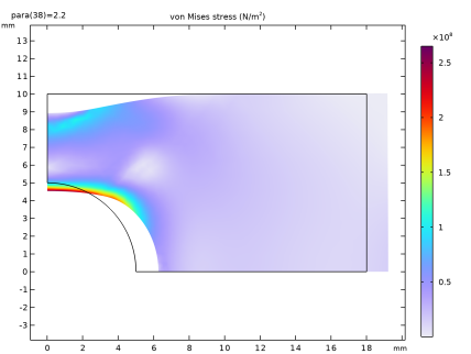
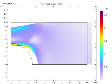
In the Settings window for 2D Plot Group, type Stress, Interpolated Hardening and User-Defined Plastic Flow in the Label text field.
3
Locate the Data section. From the Dataset list, choose Interpolated Hardening and User-Defined Plastic Flow/Solution 2 (sol2).
4
In the Stress, Interpolated Hardening and User-Defined Plastic Flow toolbar, click  Plot.
5
Click the  Zoom Extents button in the Graphics toolbar.
Plastic Region, Interpolated Hardening and User-Defined Plastic Flow
1
In the Model Builder window, right-click Plastic Region, Linear Hardening and choose Duplicate.
2
In the Settings window for 2D Plot Group, type Plastic Region, Interpolated Hardening and User-Defined Plastic Flow in the Label text field.
3
Locate the Data section. From the Dataset list, choose Interpolated Hardening and User-Defined Plastic Flow/Solution 2 (sol2).
4
In the Plastic Region, Interpolated Hardening and User-Defined Plastic Flow toolbar, click  Plot.
Surface 1
1
In the Model Builder window, expand the Plastic Region, Interpolated Hardening and User-Defined Plastic Flow node, then click Surface 1.
2
Plastic Region, Interpolated Hardening and User-Defined Plastic Flow
Click the  Zoom Extents button in the Graphics toolbar.
The analysis is now finished. If you want to store this model and reuse it later, you will need to disable the second plasticity feature for the first study.
Linear Hardening
Step 1: Stationary
1
In the Model Builder window, under Linear Hardening click Step 1: Stationary.
2
In the Settings window for Stationary, locate the Physics and Variables Selection section.
3
Select the Modify model configuration for study step checkbox.
4
In the tree, select Component 1 (comp1) > Solid Mechanics (solid) > Linear Elastic Material 1 > Interpolated Hardening and User-Defined Plastic Flow.
5