|
|
|
|
•
|
|
•
|
|
•
|
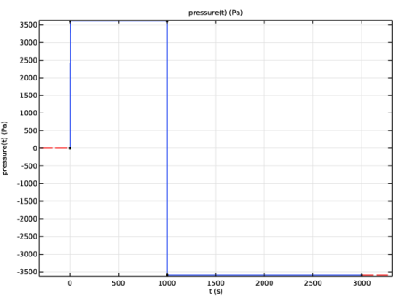
The internal pressure is ramped up from 0 to 3600 Pa during 1 s at t = 1 s and change sign within 1 s at t = 999 s as illustrated in Figure 1.
 |

|
1
|
|
2
|
|
3
|
Click Add.
|
|
4
|
Click
|
|
5
|
|
6
|
Click
|
|
1
|
|
2
|
|
1
|
|
2
|
|
3
|
|
5
|
|
6
|
In the Function table, enter the following settings:
|
|
7
|
Click
|
|
1
|
|
2
|
|
3
|
Locate the Definition section. In the Expression text field, type 500*t^((r-7e-2)/9e-2)*(t<=0.1)+50*t^((r-0.16)/9e-2)*(t>0.1)*(t<=1)+50*(t>1).
|
|
4
|
|
5
|
Locate the Units section. In the table, enter the following settings:
|
|
6
|
|
1
|
|
2
|
|
3
|
|
4
|
Click
|
|
5
|
Browse to the model’s Application Libraries folder and double-click the file elastoplastic_creep_target.txt.
|
|
6
|
Click
|
|
7
|
Locate the Data Column Settings section. In the table, enter the following settings:
|
|
9
|
|
11
|
|
13
|
|
15
|
|
17
|
|
1
|
|
2
|
|
3
|
|
4
|
|
5
|
|
6
|
Click
|
|
1
|
|
2
|
|
3
|
From the list, choose Quasistatic.
|
|
1
|
|
2
|
|
3
|
|
4
|
|
1
|
|
2
|
|
3
|
Find the Expression for remaining selection subsection. In the Volume reference temperature text field, type 0.
|
|
1
|
|
2
|
|
3
|
|
1
|
|
2
|
|
3
|
|
4
|
|
5
|
|
6
|
|
7
|
|
8
|
|
9
|
|
1
|
|
2
|
In the Show More Options dialog, in the tree, select the checkbox for the node Physics > Advanced Physics Options.
|
|
3
|
Click OK.
|
|
4
|
|
5
|
|
6
|
|
1
|
|
3
|
|
4
|
|
1
|
|
3
|
|
4
|
|
1
|
In the Model Builder window, under Component 1 (comp1) right-click Materials and choose Blank Material.
|
|
2
|
|
4
|
In the Model Builder window, expand the Material 1 (mat1) node, then click Elastoplastic material model (ElastoplasticModel).
|
|
5
|
|
6
|
Click
|
|
7
|
|
8
|
|
9
|
Click OK.
|
|
1
|
|
2
|
|
3
|
|
5
|
|
6
|
In the Function table, enter the following settings:
|
|
1
|
|
3
|
|
4
|
|
1
|
|
3
|
|
4
|
|
5
|
Click
|
|
1
|
|
2
|
|
3
|
In the Output times text field, type 0 0.01 0.06 0.1 range(0.4, 0.2, 2) 10 50 100 200 500 range(999, 0.2, 1000) 1002 1004 1010 1025 1050 1100 1160 range(1200, 100, 1500) 2000 3000.
|
|
1
|
|
2
|
|
3
|
|
1
|
|
2
|
|
3
|
|
1
|
|
2
|
|
3
|
|
4
|
|
1
|
|
2
|
|
3
|
|
4
|
|
5
|
|
1
|
|
2
|
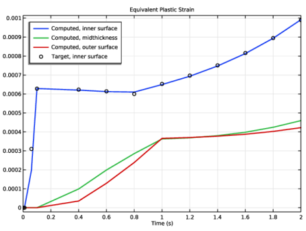
In the Settings window for Point Graph, click Replace Expression in the upper-right corner of the y-Axis Data section. From the menu, choose Component 1 (comp1) > Solid Mechanics > Strain > solid.epeGp - Equivalent plastic strain - 1.
|
|
3
|
|
4
|
|
5
|
|
1
|
|
2
|
|
4
|
Click to expand the Coloring and Style section. Find the Line style subsection. From the Line list, choose None.
|
|
5
|
|
6
|
|
7
|
|
9
|
|
1
|
|
2
|
|
3
|
Select the Manual axis limits checkbox.
|
|
4
|
|
5
|
|
6
|
|
1
|
|
2
|
|
3
|
|
1
|
|
2
|
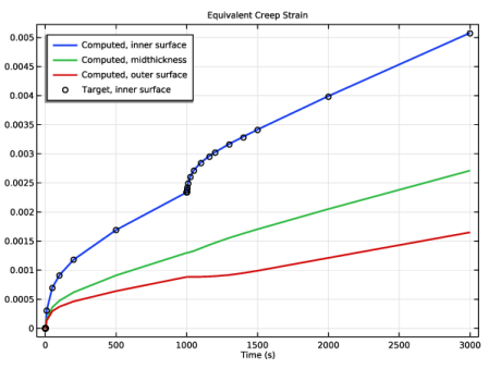
In the Settings window for Point Graph, click Replace Expression in the upper-right corner of the y-Axis Data section. From the menu, choose Component 1 (comp1) > Solid Mechanics > Strain > solid.eceGp - Equivalent creep strain - 1.
|
|
1
|
|
2
|
|
4
|
|
1
|
|
2
|
|
3
|
|
4
|
|
1
|
|
2
|
|
3
|
|
4
|
|
1
|
|
2
|
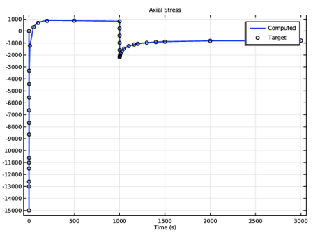
In the Settings window for Point Graph, click Replace Expression in the upper-right corner of the y-Axis Data section. From the menu, choose Component 1 (comp1) > Solid Mechanics > Stress > Stress tensor (spatial frame) - N/m² > solid.sGpzz - Stress tensor, zz-component.
|
|
3
|
Locate the Legends section. In the table, enter the following settings:
|
|
1
|
|
2
|
|
4
|
Locate the Legends section. In the table, enter the following settings:
|
|
5
|
|
1
|
|
2
|
|
1
|
|
2
|
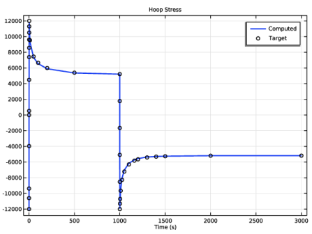
In the Settings window for Point Graph, click Replace Expression in the upper-right corner of the y-Axis Data section. From the menu, choose Component 1 (comp1) > Solid Mechanics > Stress > Stress tensor (spatial frame) - N/m² > solid.sGpphiphi - Stress tensor, phiphi-component.
|
|
1
|
|
2
|
|
4
|
|
1
|
|
2
|
|
1
|
|
2
|
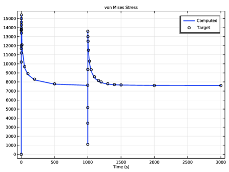
In the Settings window for Point Graph, click Replace Expression in the upper-right corner of the y-Axis Data section. From the menu, choose Component 1 (comp1) > Solid Mechanics > Stress > solid.misesGp - von Mises stress - N/m².
|
|
1
|
|
2
|
|
4
|
|
1
|
|
2
|
|
3
|
|
1
|
|
2
|
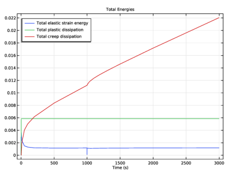
In the Settings window for Global, click Add Expression in the upper-right corner of the y-Axis Data section. From the menu, choose Component 1 (comp1) > Solid Mechanics > Global > solid.Ws_tot - Total elastic strain energy - J.
|
|
3
|
Click Add Expression in the upper-right corner of the y-Axis Data section. From the menu, choose Component 1 (comp1) > Solid Mechanics > Global > solid.Wp_tot - Total plastic dissipation - J.
|
|
4
|
Click Add Expression in the upper-right corner of the y-Axis Data section. From the menu, choose Component 1 (comp1) > Solid Mechanics > Global > solid.Wc_tot - Total creep dissipation - J.
|
|
1
|
|
2
|
|
3
|
|
4
|