
|
|
|
|
1
|
|
2
|
|
3
|
Click Add.
|
|
4
|
Click
|
|
5
|
|
6
|
Click
|
|
1
|
|
2
|
Browse to the model’s Application Libraries folder and double-click the file diaphragm_accumulator_geom_sequence.mph.
|
|
1
|
|
2
|
|
1
|
|
2
|
|
3
|
Locate the Parameters section. In the table, enter the following settings:
|
|
1
|
|
2
|
|
3
|
|
5
|
Locate the Interpolation and Extrapolation section. From the Interpolation list, choose Piecewise cubic.
|
|
6
|
|
7
|
In the Argument table, enter the following settings:
|
|
8
|
Click
|
|
1
|
|
2
|
|
3
|
Click
|
|
4
|
|
5
|
Click OK.
|
|
6
|
|
7
|
Click
|
|
8
|
|
9
|
Click OK.
|
|
1
|
In the Model Builder window, under Component 1 (comp1) > Solid Mechanics (solid) click Linear Elastic Material 1.
|
|
1
|
|
2
|
|
3
|
Click
|
|
5
|
|
1
|
|
2
|
|
3
|
|
4
|
|
1
|
|
2
|
|
3
|
|
4
|
|
1
|
|
1
|
|
2
|
In the Settings window for Enclosed Cavity, type Enclosed Cavity, Nitrogen Gas in the Label text field.
|
|
3
|
|
4
|
In the Paste Selection dialog, type 5, 9, 10, 16, 34-36, 40-42, 47, 52, 55, 59, 66, 67, 69, 70, 73, 75 in the Selection text field.
|
|
5
|
Click OK.
|
|
6
|
|
7
|
|
8
|
|
1
|
|
2
|
|
3
|
|
1
|
|
2
|
|
3
|
|
4
|
|
1
|
|
2
|
In the Settings window for Enclosed Cavity, type Enclosed Cavity, Hydraulic Fluid in the Label text field.
|
|
3
|
|
4
|
|
6
|
|
7
|
|
8
|
Click OK.
|
|
1
|
|
2
|
|
3
|
|
1
|
|
2
|
Go to the Add Material window.
|
|
3
|
|
4
|
Right-click and choose Add to Component 1 (comp1).
|
|
5
|
|
1
|
|
2
|
|
1
|
|
2
|
|
3
|
|
4
|
Locate the Material Contents section. In the table, enter the following settings:
|
|
1
|
In the Model Builder window, expand the Component 1 (comp1) > Materials > Nitrile butadiene rubber (NBR) (mat2) node.
|
|
2
|
|
3
|
|
4
|
|
5
|
Locate the Material Contents section. In the table, enter the following settings:
|
|
1
|
|
2
|
|
3
|
|
5
|
|
1
|
|
2
|
|
3
|
|
5
|
|
6
|
Locate the Element Size Parameters section.
|
|
7
|
|
8
|
|
1
|
|
2
|
|
3
|
|
5
|
Locate the Element Size Expression section. In the Size expression text field, type if(R>10[mm], 0.22, 0.5)*dia.th.
|
|
1
|
|
3
|
|
4
|
|
5
|
Click
|
|
1
|
|
2
|
|
1
|
|
2
|
|
3
|
Select the Modify model configuration for study step checkbox.
|
|
4
|
In the tree, select Component 1 (comp1) > Solid Mechanics (solid), Controls spatial frame > Enclosed Cavity, Nitrogen Gas > Fluid 1 and Component 1 (comp1) > Solid Mechanics (solid), Controls spatial frame > Enclosed Cavity, Hydraulic Fluid > Prescribed Pressure 1.
|
|
5
|
Right-click and choose Disable.
|
|
6
|
|
7
|
Click
|
|
9
|
|
1
|
|
2
|
|
3
|
Click
|
|
4
|
|
5
|
Click OK.
|
|
6
|
|
8
|
Click
|
|
1
|
|
2
|
|
1
|
|
2
|
|
3
|
|
4
|
|
5
|
|
1
|
|
2
|
|
3
|
|
4
|
|
1
|
|
2
|
|
1
|
|
2
|
Go to the Add Study window.
|
|
3
|
|
4
|
Right-click and choose Add Study.
|
|
5
|
|
1
|
|
2
|
|
3
|
|
4
|
Click to expand the Values of Dependent Variables section. Find the Initial values of variables solved for subsection. From the Settings list, choose User controlled.
|
|
5
|
|
6
|
|
7
|
|
1
|
|
2
|
|
3
|
|
4
|
|
5
|
|
6
|
In the Model Builder window, expand the Hydraulic Fluid > Solver Configurations > Solution 2 (sol2) > Time-Dependent Solver 1 node, then click Fully Coupled 1.
|
|
7
|
|
8
|
|
9
|
|
10
|
Click
|
|
1
|
|
2
|
|
1
|
|
2
|
|
3
|
|
4
|
|
5
|
|
1
|
|
2
|
|
3
|
|
4
|
|
1
|
|
2
|
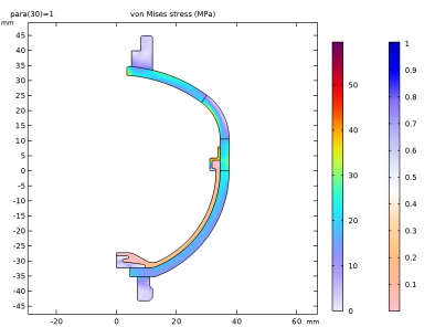
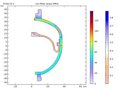
In the Settings window for 3D Plot Group, type Stress, 3D (Hydraulic Fluid) in the Label text field.
|
|
1
|
In the Model Builder window, expand the Hydraulic Fluid > Solver Configurations > Solution 2 (sol2) > Time-Dependent Solver 1 node.
|
|
2
|
|
3
|
|
4
|
Click to expand the Title section. Locate the Data section. From the Dataset list, choose Hydraulic Fluid/Solution 2 (sol2).
|
|
5
|
|
6
|
Locate the Plot Settings section.
|
|
7
|
|
1
|
|
2
|
|
4
|
|
1
|
|
2
|
|
3
|
|
4
|
|
5
|
|
1
|
|
2
|
|
4
|
|
1
|
|
2
|
|
3
|
|
4
|
|
5
|
|
6
|
|
7
|
|
1
|
|
2
|
|
1
|
|
2
|
|
3
|
Click
|
|
5
|
|
1
|
|
2
|
|
3
|
|
4
|
|
5
|
|
6
|
|
1
|
|
2
|
|
3
|
|
1
|
|
2
|
|
3
|
|
4
|
|
1
|
|
2
|
|
3
|
|
1
|
|
1
|
|
2
|
|
3
|
|
4
|
|
1
|
|
2
|
|
3
|
|
1
|
|
2
|
|
3
|
|
4
|
|
1
|
|
2
|
|
3
|
|
1
|
|
2
|
|
3
|
|
4
|
|
5
|
In the Settings window for 3D Plot Group, in the Graphics window toolbar, click
|
|
6
|
|
7
|
|
8
|
|
9
|
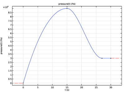
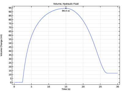
 Volume of hydraulic fluid entering the accumulator.