
|
|
|
|
•
|
Young’s modulus is 30 GPa.
|
|
•
|
Poisson’s ratio is 0.2.
|
|
•
|
The tensile strength is 2 MPa.
|
|
•
|
The fracture energy is 60 J/m2. This is the energy dissipated during the creation of a single crack. The cracking process is modeled using an isotropic damage model with a single damage variable that only considers the tensile failure of the material.
|
|
1
|
|
2
|
|
3
|
Click Add.
|
|
4
|
Click
|
|
5
|
|
6
|
Click
|
|
1
|
|
2
|
|
1
|
|
2
|
|
3
|
|
1
|
|
2
|
|
3
|
|
4
|
|
5
|
Click
|
|
1
|
|
2
|
|
3
|
From the list, choose Plane stress.
|
|
4
|
|
1
|
|
2
|
|
1
|
|
2
|
|
3
|
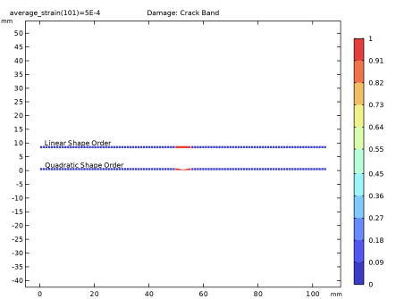
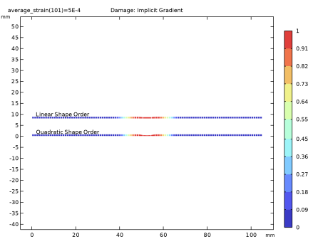
Locate the Damage section. Find the Spatial regularization method subsection. From the list, choose Implicit gradient.
|
|
4
|
|
5
|
|
1
|
In the Model Builder window, under Component 1 (comp1) right-click Materials and choose Blank Material.
|
|
2
|
|
1
|
|
2
|
Right-click Component 1 (comp1) > Materials > Material 1 (mat1) > Scalar damage (sdmg) and choose Functions > Piecewise.
|
|
3
|
|
4
|
|
5
|
Locate the Definition section. Find the Intervals subsection. In the table, enter the following settings:
|
|
6
|
|
7
|
|
1
|
In the Model Builder window, under Component 1 (comp1) > Materials > Material 1 (mat1) click Scalar damage (sdmg).
|
|
2
|
|
1
|
|
1
|
|
3
|
|
4
|
|
5
|
|
1
|
|
3
|
|
4
|
|
1
|
|
2
|
|
1
|
|
2
|
|
3
|
Select the Auxiliary sweep checkbox.
|
|
4
|
Click
|
|
6
|
Locate the Physics and Variables Selection section. Select the Modify model configuration for study step checkbox.
|
|
7
|
In the tree, select Component 1 (comp1) > Solid Mechanics (solid) > Linear Elastic Material 1 > Damage: Implicit Gradient.
|
|
8
|
Right-click and choose Disable.
|
|
1
|
|
2
|
|
3
|
In the Model Builder window, expand the Crack Band, Quadratic > Solver Configurations > Solution 1 (sol1) > Stationary Solver 1 node, then click Parametric 1.
|
|
4
|
|
5
|
Select the Tuning of step size checkbox.
|
|
6
|
|
7
|
|
8
|
|
9
|
In the Model Builder window, under Crack Band, Quadratic > Solver Configurations > Solution 1 (sol1) click Dependent Variables 1.
|
|
10
|
|
11
|
|
12
|
|
13
|
|
1
|
|
2
|
|
3
|
Click
|
|
4
|
|
5
|
Click OK.
|
|
6
|
|
8
|
Click
|
|
9
|
|
10
|
Click OK.
|
|
11
|
|
13
|
Click
|
|
1
|
|
2
|
Go to the Result Templates window.
|
|
3
|
|
4
|
Click the Add Result Template button in the window toolbar.
|
|
5
|
|
1
|
|
2
|
|
3
|
|
1
|
|
2
|
|
3
|
|
1
|
|
2
|
|
3
|
|
1
|
|
2
|
|
3
|
|
4
|
|
5
|
|
1
|
|
2
|
|
1
|
|
2
|
Go to the Add Study window.
|
|
3
|
|
4
|
Right-click and choose Add Study.
|
|
5
|
|
1
|
|
2
|
Select the Auxiliary sweep checkbox.
|
|
3
|
Click
|
|
1
|
|
2
|
|
3
|
In the Model Builder window, expand the Study 2 > Solver Configurations > Solution 2 (sol2) > Stationary Solver 1 node, then click Parametric 1.
|
|
4
|
|
5
|
Select the Tuning of step size checkbox.
|
|
6
|
|
7
|
|
8
|
|
9
|
In the Model Builder window, under Study 2 > Solver Configurations > Solution 2 (sol2) click Dependent Variables 1.
|
|
10
|
|
11
|
|
12
|
|
13
|
|
14
|
|
15
|
Clear the Generate default plots checkbox.
|
|
16
|
|
17
|
|
18
|
|
19
|
In the Show More Options dialog, in the tree, select the checkbox for the node Physics > Advanced Physics Options.
|
|
20
|
Click OK.
|
|
1
|
|
2
|
|
3
|
|
4
|
|
1
|
|
2
|
Go to the Add Study window.
|
|
3
|
|
4
|
Right-click and choose Add Study.
|
|
5
|
|
1
|
|
2
|
Select the Auxiliary sweep checkbox.
|
|
3
|
Click
|
|
5
|
Locate the Physics and Variables Selection section. Select the Modify model configuration for study step checkbox.
|
|
6
|
In the tree, select Component 1 (comp1) > Solid Mechanics (solid) > Linear Elastic Material 1 > Damage: Implicit Gradient.
|
|
7
|
Right-click and choose Disable.
|
|
8
|
|
9
|
|
1
|
|
2
|
|
3
|
In the Model Builder window, expand the Study 3 > Solver Configurations > Solution 3 (sol3) > Stationary Solver 1 node, then click Parametric 1.
|
|
4
|
|
5
|
Select the Tuning of step size checkbox.
|
|
6
|
|
7
|
|
8
|
|
9
|
In the Model Builder window, under Study 3 > Solver Configurations > Solution 3 (sol3) click Dependent Variables 1.
|
|
10
|
|
11
|
|
12
|
|
13
|
|
14
|
|
15
|
Clear the Generate default plots checkbox.
|
|
16
|
|
17
|
|
1
|
|
2
|
Go to the Add Study window.
|
|
3
|
|
4
|
Right-click and choose Add Study.
|
|
5
|
|
1
|
|
2
|
Select the Modify model configuration for study step checkbox.
|
|
3
|
|
4
|
|
5
|
|
6
|
Click
|
|
1
|
|
2
|
|
3
|
In the Model Builder window, expand the Study 4 > Solver Configurations > Solution 4 (sol4) > Stationary Solver 1 node, then click Parametric 1.
|
|
4
|
|
5
|
Select the Tuning of step size checkbox.
|
|
6
|
|
7
|
|
8
|
|
9
|
In the Model Builder window, under Study 4 > Solver Configurations > Solution 4 (sol4) click Dependent Variables 1.
|
|
10
|
|
11
|
|
12
|
|
13
|
|
14
|
|
15
|
Clear the Generate default plots checkbox.
|
|
16
|
|
17
|
|
1
|
|
2
|
|
3
|
|
4
|
|
5
|
|
6
|
|
1
|
In the Model Builder window, under Results > Damage: Crack Band, Ctrl-click to select Surface 1, Mesh 1, and Annotation 1.
|
|
2
|
Right-click and choose Duplicate.
|
|
1
|
|
2
|
|
3
|
|
1
|
|
2
|
|
3
|
|
1
|
|
2
|
|
3
|
|
1
|
|
2
|
|
3
|
|
1
|
|
2
|
|
3
|
|
4
|
|
5
|
|
6
|
|
1
|
|
2
|
|
3
|
Locate the Data section. From the Dataset list, choose Implicit Gradient, Quadratic/Solution 2 (sol2).
|
|
1
|
|
2
|
|
3
|
|
1
|
|
2
|
|
3
|
|
4
|
|
1
|
|
2
|
|
1
|
|
2
|
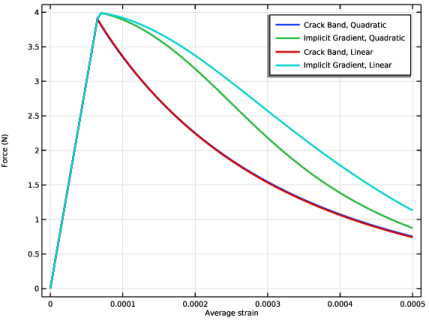
In the Settings window for Global, click Replace Expression in the upper-right corner of the y-Axis Data section. From the menu, choose Component 1 (comp1) > Solid Mechanics > Reactions > Prescribed Displacement 1 > Reaction force (spatial frame) - N > solid.disp1.RFsumx - Reaction force, x-component.
|
|
3
|
Locate the y-Axis Data section. In the table, enter the following settings:
|
|
4
|
|
5
|
|
1
|
|
2
|
|
3
|
|
4
|
Locate the Legends section. In the table, enter the following settings:
|
|
1
|
|
2
|
|
3
|
|
4
|
Locate the Legends section. In the table, enter the following settings:
|
|
1
|
|
2
|
|
3
|
|
4
|
Locate the Legends section. In the table, enter the following settings:
|
|
1
|
|
2
|
|
3
|
|
4
|
Locate the Plot Settings section.
|
|
5
|
|
6
|
|
1
|
|
2
|
|
3
|
|
4
|
|
5
|
|
1
|
|
2
|
|
3
|
Locate the Data section. From the Dataset list, choose Implicit Gradient, Quadratic/Solution 2 (sol2).
|
|
1
|
|
2
|
|
3
|
|
1
|
|
2
|
|
3
|
|
1
|
|
2
|
|
3
|
|
1
|
|
2
|
|
3
|
|
4
|
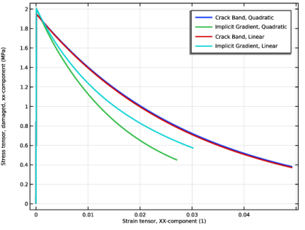
Click Replace Expression in the upper-right corner of the y-Axis Data section. From the menu, choose Component 1 (comp1) > Solid Mechanics > Damage > Stress tensor, damaged (spatial frame) - N/m² > solid.sdGpxx - Stress tensor, damaged, xx-component.
|
|
5
|
|
6
|
Click Replace Expression in the upper-right corner of the x-Axis Data section. From the menu, choose Component 1 (comp1) > Solid Mechanics > Strain > Strain tensor (material and geometry frames) > solid.eXX - Strain tensor, XX-component.
|
|
7
|
|
8
|
|
9
|
|
10
|
|
1
|
|
2
|
|
3
|
|
4
|
Locate the Legends section. In the table, enter the following settings:
|
|
1
|
|
2
|
|
3
|
|
4
|
Locate the Legends section. In the table, enter the following settings:
|
|
1
|
|
2
|
|
3
|
|
4
|
Locate the Legends section. In the table, enter the following settings:
|
|
5
|
|
1
|
|
2
|
|
3
|
|
1
|
|
2
|
|
3
|
|
4
|
|
5
|
|
1
|
|
2
|
|
3
|
|
4
|
|
1
|
|
2
|
|
3
|
|
4
|
|
1
|
|
2
|
|
3
|
|
4
|
|
5
|
|
1
|
|
2
|
|
3
|
|
4
|
|
1
|
|
3
|
In the Settings window for Line Graph, click Replace Expression in the upper-right corner of the y-Axis Data section. From the menu, choose Component 1 (comp1) > Solid Mechanics > Damage > solid.kappadmgGp - Maximum value of equivalent strain - 1.
|
|
4
|
|
5
|
|
6
|
|
7
|
|
8
|
|
9
|
|
10
|
|
11
|
|
12
|
|
13
|
|
14
|
|
16
|
|
1
|
|
2
|
|
3
|
|
4
|
|
5
|
Locate the Legends section. In the table, enter the following settings:
|
|
6
|
|
1
|
In the Model Builder window, under Results > Localization, Quadratic, Ctrl-click to select Line Graph 1 and Line Graph 2.
|
|
2
|
Right-click and choose Duplicate.
|
|
1
|
In the Settings window for Line Graph, click Replace Expression in the upper-right corner of the y-Axis Data section. From the menu, choose Component 1 (comp1) > Solid Mechanics > Damage > solid.dmgGp - Damage - 1.
|
|
2
|
Locate the Legends section. In the table, enter the following settings:
|
|
1
|
|
2
|
|
3
|
|
4
|
Locate the Legends section. In the table, enter the following settings:
|
|
1
|
|
2
|
|
3
|
Select the Two y-axes checkbox.
|
|
4
|
|
5
|
|
1
|
|
2
|
|
3
|
|
1
|
|
2
|
|
3
|
|
1
|
|
2
|
|
3
|
|
4
|
|
1
|
|
2
|
|
3
|
|
1
|
|
2
|
|
3
|
|
4
|
Locate the Legends section. In the table, enter the following settings:
|
|
5
|
Locate the Coloring and Style section. Find the Line markers subsection. From the Positioning list, choose In evaluation points.
|
|
1
|
|
2
|
|
3
|
|
4
|
Locate the Legends section. In the table, enter the following settings:
|
|
5
|
Locate the Coloring and Style section. Find the Line markers subsection. From the Positioning list, choose In evaluation points.
|
|
1
|
|
2
|
|
3
|
|
4
|
|
5
|
|
6
|
Locate the Legends section. In the table, enter the following settings:
|
|
7
|
Locate the Coloring and Style section. Find the Line markers subsection. From the Positioning list, choose In evaluation points.
|
|
1
|
|
2
|
|
3
|
|
4
|
|
5
|
Locate the Legends section. In the table, enter the following settings:
|
|
6
|
Locate the Coloring and Style section. Find the Line markers subsection. From the Positioning list, choose In evaluation points.
|
|
1
|
|
2
|
|
3
|
Select the Manual axis limits checkbox.
|
|
4
|
|
5
|
|
6
|
|
7
|