PDF

Indentation of a Cylindrical Battery Cell
Introduction
This study investigates the mechanical response of a cylindrical battery cell in the well-known 18650 format subjected to an indentation test. The test setup consists of a cylindrical indenter, whose axis is perpendicular to that of the battery cell, pressed into the cell. On the opposite side, the cell rests on a flat plate. The objective of the study is to demonstrate the use of an explicit dynamics analysis that accounts for contact mechanics and plastic deformation, and to highlight recommended settings for such simulations.
Model Definition
The battery cell is composed of a jelly roll wound around a central core and enclosed within a thin-walled cylindrical can with a cap. The can has an outer diameter of D = 18 mm, a height of H = 65 mm, and a wall thickness of t = 0.6 mm.
Due to the symmetry of both the geometry and the loading conditions, the problem can be simplified by modeling only half of the cell, along with the indenter and the support plate, using the xz-plane as the symmetry plane.
The jelly roll consists of multiple layers of different materials. For this example, it is treated as a homogenized Hyperelastic Material combined with a pressure-dependent plasticity model. The can, core, and cap are metallic components and are therefore modeled as a Linear Elastic Material with an additional plasticity model to capture permanent deformation.
Because the indenter is significantly stiffer than the battery cell, it is modeled as a rigid body. Its motion is prescribed by a Prescribed Displacement, with the indenter penetrating into the cell by 8 mm.
Accurate representation of the contact between the indenter, cell, and plate requires very small time steps. This motivates the use of explicit dynamics analysis, which is well-suited for such problems due to its ability to handle small, stable time steps with relatively low computational cost per step. Computational efficiency is further improved by employing reduced integration.
However, reduced integration can introduce spurious hourglass modes in the finite element solution. To suppress these unphysical deformations, a stabilization scheme is applied.
The maximum stable time step in explicit dynamics is proportional to the smallest element size for constant density and stiffness. Consequently, a few very small elements can significantly reduce the overall time step. To prevent excessive computational cost, artificial mass scaling is applied to these smallest elements, allowing the use of a target stable time step.
It is recommended to always assess the influence of a stabilization scheme and the artificially added mass on the computed solution.
Results and Discussion
Figure 1 visualizes the pressure pm inside of the jelly roll at the end of the indentation process. The pressure is evaluated as
with the Cauchy stress tensor σ.
Figure 1: Pressure in the jelly roll at the end of the indentation process.
Figure 2 shows the equivalent plastic strain at the end of the indentation process. The plastic strain exceeds 70% at the center of the cylindrical battery cell.
Figure 2: Equivalent plastic strain at the end of the indentation process.
Figure 3 shows the evolution of the reaction force experienced by the indenter as a function of its vertical displacement. As the indentation progresses, both the reaction force and particularly its slope increase. This behavior is attributed to the growing contact area between the cylindrical battery cell and the indenter, which leads to a greater mechanical resistance of the cell against further indentation.
Figure 3: Development of the reaction force in the indenter over the displacement of the indenter.
For the used explicit dynamics analysis with stabilization against hourglass modes and artificially added mass, it is recommended to compare the energies introduced by these methods with physically meaningful energies. Figure 4 compares the different energies occurring in this study over time. Most prominently, it can be seen that most of the energy is dissipated due to the plastic deformations inside of the battery cell, while a comparably minor amount of the energy is stored elastically. The total kinetic energy is almost zero meaning that the given example behaves quasi-static. In this example, the total artificial kinetic energy and the total stabilization energy are of particular interest with the first being an indicator of the influence of the Mass Scaling on the computed result and the second of the stabilization scheme. First, it can be seen that the total artificial kinetic energy is almost zero, like the physically meaningful total kinetic energy. From this, it can be concluded that the Mass Scaling does not drastically influence the computed results. Second, it can be seen that also the total stabilization strain energy consumes only a minor amount of the energy compared to the physically meaningful dissipated energy and the elastic strain energy. This leads to the conclusion that the computed results are also not critically influenced by the stabilization scheme.
Figure 4: Development of the different energies over time.
Although it was found that the Mass Scaling did not deteriorate the computed results, it is still a good habit to check which elements contain artificially added mass and to which extent mass was added. Thus, in Figure 5, the ratio of the artificially added mass density and the physically meaningful mass density is shown. Note that the values are element specific. It can be seen that mass is added where elements are small, have a small aspect ratio, or where the material features a stiff behavior. In this example this is mainly in the can of the battery cell with a small wall thickness and a large Young’s modulus.
Figure 5: Ratio of artificial mass density and actual mass density.
Notes About the COMSOL Implementation
Consider the following when setting up the model:
The vertical movement of the indenter is modeled by Prescribed Displacement node. This represents a perfectly stiff body.
To circumvent the need to specify potential contact boundaries between the different components, a General Contact Pair is used in which contact mechanics is considered between all domains.
Application Library path: Nonlinear_Structural_Materials_Module/Plasticity/cylindrical_battery_indentation
Modeling Instructions
From the File menu, choose New.
New
In the New window, click  Model Wizard.
Model Wizard
1
In the Model Wizard window, click  3D.
2
In the Select Physics tree, select Structural Mechanics > Explicit Dynamics > Solid Mechanics, Explicit Dynamics (solid).
3
Click Add.
4
Click  Study.
5
In the Select Study tree, select Preset Studies for Selected Physics Interfaces > Explicit Dynamics.
6
Global Definitions
Parameters 1
1
In the Model Builder window, under Global Definitions click Parameters 1.
2
In the Settings window for Parameters, locate the Parameters section.
3
Click the Load button. From the menu, choose Load from File.
4
Geometry 1
1
In the Geometry toolbar, click Insert Sequence and choose Insert Sequence.
2
Complete geometry instructions can be found in the Appendix — Geometry Modeling Instructions section. Note that the geometric symmetry and the symmetry of the applied load is utilized and the geometry is cut at the zx-plane.
Definitions
Create a General Contact Pair node to include contact between all surfaces. The cap and the core of the battery cell are glued to the shell and the jelly roll, respectively. Model this through a continuity condition by adding an Identity Boundary Pair.
General Contact Pair 1 (p1)
1
In the Model Builder window, expand the Component 1 (comp1) > Definitions node.
2
Right-click Definitions and choose Pairs > General Contact Pair.
Identity Boundary Pair 2 (p2)
1
In the Definitions toolbar, click  Pairs and choose Identity Boundary Pair.
2
In the Settings window for Pair, locate the Source Boundaries section.
3
Click to select the  Activate Selection toggle button.
4
5
Locate the Destination Boundaries section. Click to select the  Activate Selection toggle button.
6
7
Locate the Frame section. From the Source frame list, choose Material  (X, Y, Z).
8
From the Destination frame list, choose Material  (X, Y, Z).
Solid Mechanics, Explicit Dynamics (solid)
1
In the Model Builder window, under Component 1 (comp1) click Solid Mechanics, Explicit Dynamics (solid).
2
3
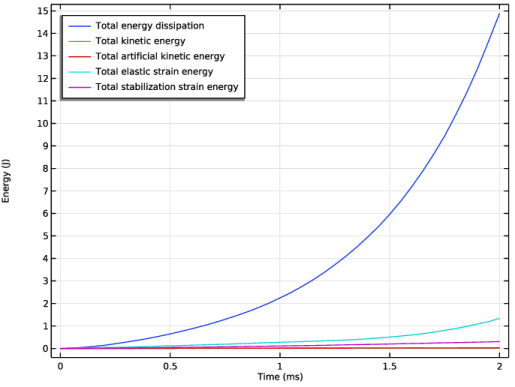
In the Settings window for Solid Mechanics, Explicit Dynamics, click to expand the Energy Dissipation section.
4
From the Store dissipation list, choose Total.
Linear Elastic Material 1
In the Model Builder window, under Component 1 (comp1) > Solid Mechanics, Explicit Dynamics (solid) click Linear Elastic Material 1.
Plasticity 1
1
In the Physics toolbar, click  Attributes and choose Plasticity.
2
3
In the Settings window for Plasticity, locate the Plasticity Model section.
4
Find the Isotropic hardening model subsection. From the list, choose Swift.
Hyperelastic Material 1
1
In the Physics toolbar, click  Domains and choose Hyperelastic Material.
2
3
In the Settings window for Hyperelastic Material, locate the Hyperelastic Material section.
4
From the Specify list, choose Young’s modulus and Poisson’s ratio.
Pressure-Dependent Plasticity 1
1
In the Physics toolbar, click  Attributes and choose Pressure-Dependent Plasticity.
2
In the Settings window for Pressure-Dependent Plasticity, locate the Plasticity Model section.
3
Define a contact model including friction between all domains.
Contact Model 1
1
In the Model Builder window, expand the Component 1 (comp1) > Solid Mechanics, Explicit Dynamics (solid) > General Contact 1 node, then click Contact Model 1.
2
In the Settings window for Contact Model, locate the Contact Model section.
3
From the Penalty factor multiplier list, choose Manual tuning.
Friction 1
1
In the Physics toolbar, click  Attributes and choose Friction.
2
In the Settings window for Friction, locate the Friction Parameters section.
3
In the μ text field, type 0.3.
Add a Mass Scaling node to automatically add artificial localized mass to increase the size of the stable time step of the explicit dynamics analysis.
Mass Scaling 1
1
In the Physics toolbar, click  Domains and choose Mass Scaling.
2
In the Settings window for Mass Scaling, locate the Domain Selection section.
3
From the Selection list, choose All domains.
4
Locate the Mass Scaling section. In the Δtcell0 text field, type 3e-8.
Add a symmetry condition at the zx-plane to respect the symmetry cut in the geometry.
Symmetry 1
1
In the Physics toolbar, click  Boundaries and choose Symmetry.
2
Prescribed Displacement 1
1
In the Physics toolbar, click  Domains and choose Prescribed Displacement.
2
In the Settings window for Prescribed Displacement, locate the Prescribed Displacement section.
3
Specify the u0 vector as
4
Materials
Can
1
In the Model Builder window, under Component 1 (comp1) right-click Materials and choose Blank Material.
2
In the Settings window for Material, type Can in the Label text field.
3
Locate the Geometric Entity Selection section. From the Selection list, choose Manual.
4
5
Locate the Material Contents section. In the table, enter the following settings:
Jelly Roll
1
Right-click Materials and choose Blank Material.
2
In the Settings window for Material, type Jelly Roll in the Label text field.
3
4
Locate the Material Contents section. In the table, enter the following settings:
Cap
1
Right-click Materials and choose Blank Material.
2
In the Settings window for Material, type Cap in the Label text field.
3
4
Locate the Material Contents section. In the table, enter the following settings:
Core
1
Right-click Materials and choose Blank Material.
2
In the Settings window for Material, type Core in the Label text field.
3
4
Locate the Material Contents section. In the table, enter the following settings:
Create a dummy material for the rigid indenter.
Indenter
1
Right-click Materials and choose Blank Material.
2
In the Settings window for Material, type Indenter in the Label text field.
3
4
Locate the Material Contents section. In the table, enter the following settings:
Mesh 1
Mapped 1
1
In the Mesh toolbar, click  More Generators and choose Mapped.
2
Distribution 1
1
Right-click Mapped 1 and choose Distribution.
2
3
In the Settings window for Distribution, locate the Distribution section.
4
In the Number of elements text field, type 1.
Distribution 2
1
In the Model Builder window, right-click Mapped 1 and choose Distribution.
2
3
In the Settings window for Distribution, locate the Distribution section.
4
In the Number of elements text field, type 2.
Free Quad 1
1
In the Mesh toolbar, click  More Generators and choose Free Quad.
2
Swept 1
1
In the Mesh toolbar, click  Swept.
2
In the Settings window for Swept, locate the Domain Selection section.
3
From the Geometric entity level list, choose Domain.
4
Distribution 1
1
Right-click Swept 1 and choose Distribution.
2
In the Settings window for Distribution, locate the Distribution section.
3
In the Number of elements text field, type 1.
4
Distribution 2
1
In the Model Builder window, right-click Swept 1 and choose Distribution.
2
In the Settings window for Distribution, locate the Distribution section.
3
In the Number of elements text field, type 2.
4
Size
1
In the Model Builder window, under Component 1 (comp1) > Mesh 1 click Size.
2
In the Settings window for Size, locate the Element Size section.
3
Click the Custom button.
4
Locate the Element Size Parameters section. In the Maximum element size text field, type 1.
5
In the Minimum element size text field, type 0.75.
Free Quad 2
1
In the Mesh toolbar, click  More Generators and choose Free Quad.
2
Swept 2
In the Mesh toolbar, click  Swept.
Study 1
Step 1: Explicit Dynamics
1
In the Model Builder window, under Study 1 click Step 1: Explicit Dynamics.
2
In the Settings window for Explicit Dynamics, locate the Study Settings section.
3
From the Time unit list, choose ms.
4
In the Output times text field, type range(0,0.05,2).
Decrease the number of updates of data structures used by the contact search algorithm. This is justified for the small deformations expected in each time step.
5
Click to expand the Results While Solving section. Select the Plot checkbox.
6
Click to expand the Explicit Dynamics Settings section. Select the Contact update frequency checkbox.
7
In the Hierarchical data text field, type 100.
8
In the Study toolbar, click  Compute.
Create a dataset that mirrors the solution at the symmetry plane for visualization.
Results
Mirror 3D 1
1
In the Results toolbar, click  More Datasets and choose Mirror 3D.
2
In the Settings window for Mirror 3D, locate the Plane Data section.
3
From the Plane list, choose ZX-planes.
4
Click to expand the Advanced section.
Preferred Units 1
1
In the Results toolbar, click  Configurations and choose Preferred Units.
2
In the Settings window for Preferred Units, locate the Units section.
3
Click  Add Physical Quantity.
4
In the Physical Quantity dialog, type stress in the text field.
5
In the tree, select Solid Mechanics > Stress tensor (N/m^2).
6
7
In the Settings window for Preferred Units, locate the Units section.
8
9
Click  Apply.
Stress (solid)
1
In the Model Builder window, under Results click Stress (solid).
2
In the Settings window for 3D Plot Group, locate the Selection section.
3
From the Geometric entity level list, choose Domain.
4
Mesh 1
Right-click Stress (solid) and choose Mesh.
Deformation 1
1
In the Model Builder window, expand the Results > Stress (solid) > Volume 1 node.
2
Right-click Mesh 1 and choose Deformation.
3
In the Settings window for Deformation, locate the Scale section.
4
Select the Scale factor checkbox. In the associated text field, type 1.
Mesh 1
1
In the Model Builder window, click Mesh 1.
2
In the Settings window for Mesh, locate the Coloring and Style section.
3
From the Element color list, choose None.
Jelly Roll Pressure
1
In the Results toolbar, click  3D Plot Group.
2
In the Settings window for 3D Plot Group, type Jelly Roll Pressure in the Label text field.
3
Locate the Data section. From the Dataset list, choose Mirror 3D 1.
4
Locate the Plot Settings section. Clear the Plot dataset edges checkbox.
5
Locate the Color Legend section. Select the Show units checkbox.
Jelly Roll
1
Right-click Jelly Roll Pressure and choose Volume.
2
In the Settings window for Volume, type Jelly Roll in the Label text field.
3
Locate the Expression section. In the Expression text field, type solid.pmGp.
4
Locate the Coloring and Style section. From the Color table list, choose Plasma.
Deformation 1
1
Right-click Jelly Roll and choose Deformation.
2
In the Settings window for Deformation, locate the Scale section.
3
Select the Scale factor checkbox. In the associated text field, type 1.
Selection 1
1
In the Model Builder window, right-click Jelly Roll and choose Selection.
2
Filter 1
1
Right-click Jelly Roll and choose Filter.
2
In the Settings window for Filter, locate the Element Selection section.
3
In the Logical expression for inclusion text field, type X<0 || Z < 0.
Transformation 1
1
Right-click Jelly Roll and choose Transformation.
2
In the Settings window for Transformation, locate the Transformation section.
3
Select the Scale checkbox.
4
In the x text field, type 0.995.
5
In the y text field, type 0.995.
6
In the z text field, type 0.995.
Can
1
In the Model Builder window, right-click Jelly Roll Pressure and choose Volume.
2
In the Settings window for Volume, type Can in the Label text field.
3
Locate the Expression section. In the Expression text field, type 1.
4
Click to expand the Title section. From the Title type list, choose None.
Deformation 1
1
Right-click Can and choose Deformation.
2
In the Settings window for Deformation, locate the Scale section.
3
Select the Scale factor checkbox. In the associated text field, type 1.
Selection 1
1
In the Model Builder window, right-click Can and choose Selection.
2
Transparency 1
1
Right-click Can and choose Transparency.
2
In the Settings window for Transparency, locate the Transparency section.
3
Find the Fresnel transmittance subsection. Set the Fresnel transmittance value to 0.5.
Results
Can
In the Model Builder window, collapse the Results > Jelly Roll Pressure > Can node.
Material Appearance 1
1
In the Model Builder window, expand the Can node.
2
Right-click Can and choose Material Appearance.
3
In the Settings window for Material Appearance, locate the Appearance section.
4
From the Appearance list, choose Custom.
5
From the Material type list, choose Steel.
Core
1
In the Model Builder window, right-click Jelly Roll Pressure and choose Volume.
2
In the Settings window for Volume, type Core in the Label text field.
3
Locate the Expression section. In the Expression text field, type 1.
4
Locate the Title section. From the Title type list, choose None.
Deformation 1
1
Right-click Core and choose Deformation.
2
In the Settings window for Deformation, locate the Scale section.
3
Select the Scale factor checkbox. In the associated text field, type 1.
Selection 1
1
In the Model Builder window, right-click Core and choose Selection.
2
Transparency 1
1
Right-click Core and choose Transparency.
2
In the Settings window for Transparency, locate the Transparency section.
3
Find the Fresnel transmittance subsection. In the Fresnel transmittance text field, type 0.5.
Material Appearance 1
1
Right-click Core and choose Material Appearance.
2
In the Settings window for Material Appearance, locate the Appearance section.
3
From the Appearance list, choose Custom.
4
From the Material type list, choose Aluminum.
Cap
1
In the Model Builder window, right-click Jelly Roll Pressure and choose Volume.
2
In the Settings window for Volume, type Cap in the Label text field.
3
Locate the Expression section. In the Expression text field, type 1.
4
Locate the Title section. From the Title type list, choose None.
Deformation 1
1
Right-click Cap and choose Deformation.
2
In the Settings window for Deformation, locate the Scale section.
3
Select the Scale factor checkbox. In the associated text field, type 1.
Selection 1
1
In the Model Builder window, right-click Cap and choose Selection.
2
Transparency 1
1
Right-click Cap and choose Transparency.
2
In the Settings window for Transparency, locate the Transparency section.
3
Find the Fresnel transmittance subsection. In the Fresnel transmittance text field, type 0.5.
Material Appearance 1
1
Right-click Cap and choose Material Appearance.
2
In the Settings window for Material Appearance, locate the Appearance section.
3
From the Appearance list, choose Custom.
4
From the Material type list, choose Iron.
Indenter
1
In the Model Builder window, right-click Jelly Roll Pressure and choose Volume.
2
In the Settings window for Volume, type Indenter in the Label text field.
3
Locate the Expression section. In the Expression text field, type 1.
4
Locate the Title section. From the Title type list, choose None.
Deformation 1
1
Right-click Indenter and choose Deformation.
2
In the Settings window for Deformation, locate the Scale section.
3
Select the Scale factor checkbox. In the associated text field, type 1.
Selection 1
1
In the Model Builder window, right-click Indenter and choose Selection.
2
Material Appearance 1
1
Right-click Indenter and choose Material Appearance.
2
In the Settings window for Material Appearance, locate the Appearance section.
3
From the Appearance list, choose Custom.
4
From the Material type list, choose Carbon (forged).
Selection 1
1
In the Model Builder window, click Selection 1.
2
3
In the Jelly Roll Pressure toolbar, click  Plot.
Plate
1
In the Model Builder window, right-click Jelly Roll Pressure and choose Volume.
2
In the Settings window for Volume, type Plate in the Label text field.
3
Locate the Expression section. In the Expression text field, type 1.
4
Locate the Title section. From the Title type list, choose None.
Selection 1
1
Right-click Plate and choose Selection.
2
Material Appearance 1
1
In the Model Builder window, right-click Plate and choose Material Appearance.
2
In the Settings window for Material Appearance, locate the Appearance section.
3
From the Appearance list, choose Custom.
4
From the Material type list, choose Rock.
Reaction Force
1
In the Results toolbar, click  1D Plot Group.
2
In the Settings window for 1D Plot Group, type Reaction Force in the Label text field.
3
Locate the Legend section. Clear the Show legends checkbox.
Global 1
1
Right-click Reaction Force and choose Global.
Note, that the expression for the total reaction forces is multiplied by 2 to account for the applied symmetry condition.
2
In the Settings window for Global, locate the y-Axis Data section.
3
4
In the Description text field, type Total Reaction Force.
5
Locate the x-Axis Data section. From the Parameter list, choose Expression.
6
In the Expression text field, type indenter_velocity*t.
7
Select the Description checkbox. In the associated text field, type Indenter Displacement.
Energies
1
In the Results toolbar, click  1D Plot Group.
2
In the Settings window for 1D Plot Group, type Energies in the Label text field.
3
Locate the Plot Settings section.
4
Select the y-axis label checkbox. In the associated text field, type Energy (J).
Global 1
1
Right-click Energies and choose Global.
2
In the Settings window for Global, locate the y-Axis Data section.
3
Energies
1
In the Model Builder window, click Energies.
2
In the Settings window for 1D Plot Group, locate the Legend section.
3
From the Position list, choose Upper left.
Added Mass
1
In the Results toolbar, click  3D Plot Group.
2
In the Settings window for 3D Plot Group, type Added Mass in the Label text field.
3
Locate the Data section. From the Time (ms) list, choose 0.
4
Locate the Selection section. From the Geometric entity level list, choose Domain.
5
From the Selection list, choose All domains.
6
Volume 1
1
Right-click Added Mass and choose Volume.
2
In the Settings window for Volume, locate the Expression section.
3
In the Expression text field, type solid.rhoa/solid.rho.
4
Locate the Coloring and Style section. From the Color table transformation list, choose Reverse.
5
From the Color table type list, choose Discrete.
6
From the Color table list, choose Plasma.
Transparency 1
Right-click Volume 1 and choose Transparency.
Filter 1
1
In the Model Builder window, right-click Volume 1 and choose Filter.
2
In the Settings window for Filter, locate the Element Selection section.
3
In the Logical expression for inclusion text field, type solid.rhoa/solid.rho > 0.01.
Mesh 1
1
In the Model Builder window, right-click Added Mass and choose Mesh.
2
In the Settings window for Mesh, locate the Coloring and Style section.
3
From the Element color list, choose None.
4
From the Wireframe color list, choose Gray.
Selection 1
1
Right-click Mesh 1 and choose Selection.
2
In the Settings window for Selection, locate the Selection section.
3
From the Geometric entity level list, choose Domain.
4
From the Selection list, choose All domains.
5
Result Templates
1
In the Results toolbar, click  Result Templates to open the Result Templates window.
2
Go to the Result Templates window.
3
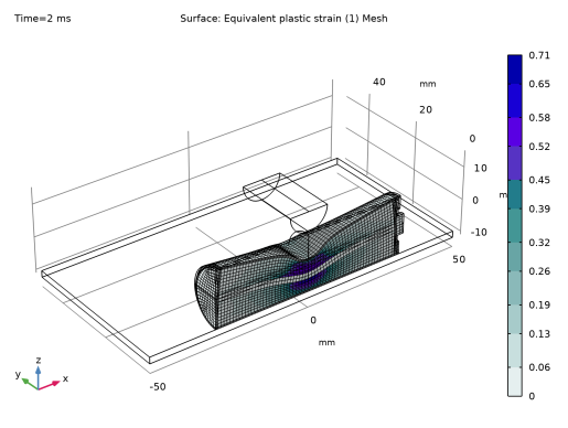
In the tree, select Study 1/Solution 1 (sol1) > Solid Mechanics, Explicit Dynamics > Equivalent Plastic Strain (solid).
4
Click the Add Result Template button in the window toolbar.
5
In the Results toolbar, click  Result Templates to close the Result Templates window.
Results
Equivalent Plastic Strain (solid)
1
In the Settings window for 3D Plot Group, locate the Selection section.
2
From the Geometric entity level list, choose Domain.
3
Deformation 1
1
In the Model Builder window, expand the Equivalent Plastic Strain (solid) node.
2
Right-click Surface 1 and choose Deformation.
3
In the Settings window for Deformation, locate the Scale section.
4
Select the Scale factor checkbox. In the associated text field, type 1.
Mesh 1
1
In the Model Builder window, right-click Equivalent Plastic Strain (solid) and choose Mesh.
2
In the Settings window for Mesh, locate the Coloring and Style section.
3
From the Element color list, choose None.
Deformation 1
1
Right-click Mesh 1 and choose Deformation.
2
In the Settings window for Deformation, locate the Scale section.
3
Select the Scale factor checkbox. In the associated text field, type 1.
Click the Zoom Box button on the Graphics toolbar and then use the mouse to zoom in and rotate the view.
Appendix — Geometry Modeling Instructions
From the File menu, choose New.
New
In the New window, click  Model Wizard.
Model Wizard
1
In the Model Wizard window, click  3D.
2
Global Definitions
Parameters 1
1
In the Model Builder window, under Global Definitions click Parameters 1.
2
In the Settings window for Parameters, locate the Parameters section.
3
Click the Load button. From the menu, choose Load from File.
4
Geometry 1
1
In the Model Builder window, under Component 1 (comp1) click Geometry 1.
2
In the Settings window for Geometry, locate the Reduction for Symmetry Boundaries section.
3
Select the zx-plane: remove y<0 checkbox.
4
Locate the Units section. From the Length unit list, choose mm.
5
Locate the Cleanup section. Clear the Automatic detection of small details checkbox.
Work Plane 1 (wp1)
1
In the Geometry toolbar, click  Work Plane.
2
In the Settings window for Work Plane, locate the Plane Definition section.
3
From the Plane list, choose yz-plane.
Work Plane 1 (wp1) > Plane Geometry
In the Model Builder window, click Plane Geometry.
Work Plane 1 (wp1) > Circle 1 (c1)
1
In the Work Plane toolbar, click  Circle.
2
In the Settings window for Circle, locate the Size and Shape section.
3
In the Radius text field, type (can_outer_diameter)/2-can_wall_thickness.
4
Click to expand the Layers section. In the table, enter the following settings:
Work Plane 1 (wp1) > Delete Entities 1 (del1)
1
Right-click Plane Geometry and choose Delete Entities.
2
In the Settings window for Delete Entities, locate the Entities or Objects to Delete section.
3
From the Geometric entity level list, choose Domain.
4
On the object c1, select Domain 5 only.
Extrude 1 (ext1)
1
In the Model Builder window, right-click Geometry 1 and choose Extrude.
2
In the Settings window for Extrude, locate the Distances section.
3
Work Plane 2 (wp2)
1
In the Geometry toolbar, click  Work Plane.
2
In the Settings window for Work Plane, locate the Plane Definition section.
3
From the Plane list, choose yz-plane.
Work Plane 2 (wp2) > Plane Geometry
In the Model Builder window, click Plane Geometry.
Work Plane 2 (wp2) > Circle 1 (c1)
1
In the Work Plane toolbar, click  Circle.
2
In the Settings window for Circle, locate the Size and Shape section.
3
In the Radius text field, type core_diameter/2.
Work Plane 2 (wp2) > Partition Domains 1 (pard1)
1
In the Work Plane toolbar, click  Booleans and Partitions and choose Partition Domains.
2
On the object c1, select Domain 1 only.
3
In the Settings window for Partition Domains, locate the Partition Domains section.
4
Click to select the  Activate Selection toggle button for Vertices defining line segments.
5
On the object c1, select Points 1 and 3 only.
Extrude 2 (ext2)
1
In the Model Builder window, right-click Geometry 1 and choose Extrude.
2
In the Settings window for Extrude, locate the Distances section.
3
Work Plane 3 (wp3)
1
In the Geometry toolbar, click  Work Plane.
2
In the Settings window for Work Plane, locate the Plane Definition section.
3
From the Plane list, choose zx-plane.
Work Plane 3 (wp3) > Plane Geometry
In the Model Builder window, click Plane Geometry.
Work Plane 3 (wp3) > Circle 1 (c1)
1
In the Work Plane toolbar, click  Circle.
2
In the Settings window for Circle, locate the Size and Shape section.
3
In the Radius text field, type indenter_diameter / 2.
4
In the Sector angle text field, type 180.
5
Locate the Rotation Angle section. In the Rotation text field, type 90.
6
Locate the Position section. In the xw text field, type can_outer_diameter / 2 + indenter_diameter / 2 +initial_gap.
Extrude 3 (ext3)
1
In the Model Builder window, right-click Geometry 1 and choose Extrude.
2
In the Settings window for Extrude, locate the Distances section.
3
Work Plane 4 (wp4)
1
In the Geometry toolbar, click  Work Plane.
2
In the Settings window for Work Plane, locate the Plane Definition section.
3
From the Plane list, choose zx-plane.
Work Plane 4 (wp4) > Plane Geometry
In the Model Builder window, click Plane Geometry.
Work Plane 4 (wp4) > Polygon 1 (pol1)
1
In the Work Plane toolbar, click  Polygon.
2
In the Settings window for Polygon, locate the Coordinates section.
3
Work Plane 4 (wp4) > Partition Domains 1 (pard1)
1
In the Work Plane toolbar, click  Booleans and Partitions and choose Partition Domains.
2
On the object pol1, select Domain 1 only.
3
In the Settings window for Partition Domains, locate the Partition Domains section.
4
Click to select the  Activate Selection toggle button for Vertices defining line segments.
5
On the object pol1, select Points 5–8 and 11–13 only.
Revolve 1 (rev1)
In the Model Builder window, right-click Geometry 1 and choose Revolve.
Work Plane 5 (wp5)
1
In the Geometry toolbar, click  Work Plane.
2
In the Settings window for Work Plane, locate the Plane Definition section.
3
From the Plane list, choose zx-plane.
Work Plane 5 (wp5) > Plane Geometry
In the Model Builder window, click Plane Geometry.
Work Plane 5 (wp5) > Polygon 1 (pol1)
1
In the Work Plane toolbar, click  Polygon.
2
In the Settings window for Polygon, locate the Coordinates section.
3
Work Plane 5 (wp5) > Partition Domains 1 (pard1)
1
In the Work Plane toolbar, click  Booleans and Partitions and choose Partition Domains.
2
On the object pol1, select Domain 1 only.
3
In the Settings window for Partition Domains, locate the Partition Domains section.
4
Click to select the  Activate Selection toggle button for Vertices defining line segments.
5
On the object pol1, select Points 3, 4, 6, and 7 only.
Revolve 2 (rev2)
In the Model Builder window, right-click Geometry 1 and choose Revolve.
Block 1 (blk1)
1
In the Geometry toolbar, click  Block.
2
In the Settings window for Block, locate the Position section.
3
From the Base list, choose Center.
4
Locate the Size and Shape section. In the Width text field, type plate_side_length.
5
In the Depth text field, type plate_side_length.
6
In the Height text field, type plate_height.
7
Locate the Position section. In the z text field, type -can_outer_diameter / 2 - plate_height / 2.
Form Union (fin)
1
In the Model Builder window, under Component 1 (comp1) > Geometry 1 click Form Union (fin).
2
In the Settings window for Form Union/Assembly, locate the Form Union/Assembly section.
3
From the Action list, choose Form an assembly.
4
Clear the Create pairs checkbox.
Form Composite Domains 1 (cmd1)
1
In the Geometry toolbar, click  Virtual Operations and choose Form Composite Domains.
2
On the object fin, select Domains 4 and 5 only.
3
In the Geometry toolbar, click  Build All.