|
|
|

|
•
|
You can find the Logarithmic option in the Geometric Nonlinearity section of the Linear Elastic Material node. Note that the computation of the Hencky strain can be further simplified by choosing the Padé option, which corresponds to the following approximation:
|
|
1
|
|
2
|
|
3
|
Click Add.
|
|
4
|
Click
|
|
5
|
|
6
|
Click
|
|
1
|
|
2
|
|
1
|
|
2
|
|
3
|
|
4
|
|
5
|
Click to expand the Layers section. In the table, enter the following settings:
|
|
1
|
|
2
|
|
3
|
|
4
|
On the object c1, select Domain 1 only.
|
|
5
|
Click
|
|
1
|
|
2
|
|
3
|
|
4
|
|
5
|
|
1
|
|
2
|
On the object r1, select Point 4 only.
|
|
3
|
|
4
|
|
1
|
|
2
|
|
3
|
|
4
|
Locate the Coordinates section. In the table, enter the following settings:
|
|
5
|
Click
|
|
1
|
|
2
|
|
3
|
|
4
|
|
5
|
|
1
|
|
3
|
|
4
|
|
1
|
In the Model Builder window, under Component 1 (comp1) right-click Materials and choose Blank Material.
|
|
2
|
|
4
|
In the Model Builder window, expand the Material 1 (mat1) node, then click Elastoplastic material model (ElastoplasticModel).
|
|
5
|
|
6
|
Click
|
|
7
|
|
8
|
|
9
|
Click OK.
|
|
1
|
|
2
|
|
3
|
Click
|
|
4
|
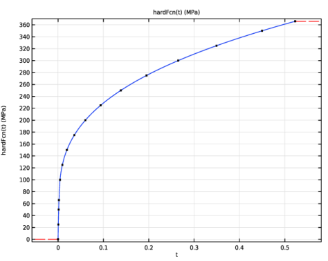
Browse to the model’s Application Libraries folder and double-click the file compressed_elastoplastic_pipe_stress_strain.txt.
|
|
5
|
|
6
|
Locate the Interpolation and Extrapolation section. From the Interpolation list, choose Piecewise cubic.
|
|
7
|
|
8
|
In the Function table, enter the following settings:
|
|
9
|
Click
|
|
1
|
|
2
|
|
1
|
|
2
|
|
3
|
|
4
|
Click OK.
|
|
1
|
|
2
|
|
4
|
|
1
|
|
2
|
|
4
|
|
1
|
|
2
|
|
3
|
|
1
|
|
2
|
|
1
|
|
1
|
|
2
|
In the Settings window for Prescribed Displacement, type Prescribed Displacement: Compression in the Label text field.
|
|
4
|
Locate the Prescribed Displacement section. From the Displacement in x direction list, choose Prescribed.
|
|
5
|
|
6
|
|
1
|
|
2
|
|
3
|
From the list, choose User-controlled mesh.
|
|
1
|
|
2
|
|
3
|
|
1
|
|
2
|
|
3
|
|
4
|
|
1
|
|
3
|
|
4
|
|
1
|
|
3
|
|
4
|
|
1
|
|
3
|
|
4
|
|
5
|
|
6
|
|
7
|
Select the Symmetric distribution checkbox.
|
|
1
|
|
1
|
|
2
|
|
3
|
|
4
|
Click
|
|
1
|
|
2
|
|
3
|
Select the Auxiliary sweep checkbox.
|
|
4
|
Click
|
|
6
|
Click to expand the Results While Solving section.
|
|
1
|
|
2
|
|
3
|
In the Model Builder window, expand the Study 1 > Solver Configurations > Solution 1 (sol1) > Stationary Solver 1 node, then click Parametric 1.
|
|
4
|
|
5
|
|
6
|
Select the Tuning of step size checkbox.
|
|
7
|
|
8
|
|
9
|
|
1
|
|
2
|
|
3
|
|
1
|
|
2
|
|
3
|
|
4
|
|
5
|
Locate the Advanced section. Find the Space variables subsection. Select the Remove elements on the symmetry axis checkbox.
|
|
1
|
|
2
|
|
3
|
|
4
|
|
1
|
|
2
|
|
3
|
|
1
|
|
2
|
Go to the Result Templates window.
|
|
3
|
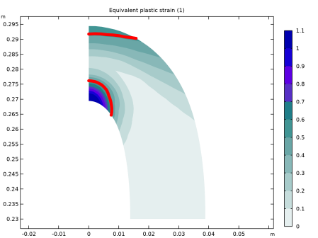
In the tree, select Study 1/Solution 1 (sol1) > Solid Mechanics > Equivalent Plastic Strain (solid) and Study 1/Solution 1 (sol1) > Solid Mechanics > Contact Forces (solid).
|
|
4
|
Click the Add Result Template button in the window toolbar.
|
|
5
|
|
1
|
|
2
|
In the Settings window for Evaluation Group, type Remaining Cross-Section Area in the Label text field.
|
|
3
|
|
1
|
|
2
|
|
4
|
|
1
|
|
2
|
|
3
|
|
4
|
|
5
|
|
1
|
|
2
|
|
3
|
|
4
|
|
1
|
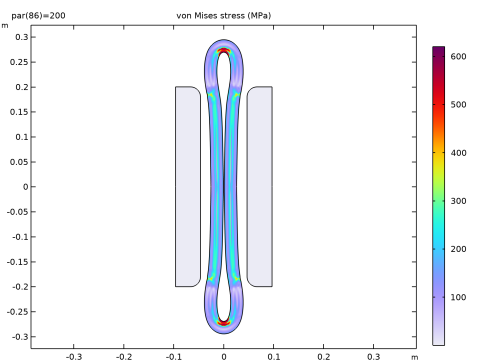
In the Model Builder window, expand the Equivalent Plastic Strain (solid) node, then click Surface 1.
|
|
2
|
|
3
|
Select the Manual color range checkbox.
|
|
4
|
|
1
|
|
2
|
|
3
|
|
1
|
|
2
|
|
3
|
|
4
|
|
5
|
|
6
|
|
7
|
|
8
|
|
9
|
Select the Radius scale factor checkbox.
|
|
10
|
|
11
|
|
12
|
Clear the Color legend checkbox.
|
|
13
|
|
14
|
Clear the Color checkbox.
|
|
1
|
|
2
|
|
3
|
|
1
|
|
2
|
|
3
|
|
4
|
Locate the Plot Settings section.
|
|
5
|
|
6
|
|
7
|
|
1
|
|
2
|
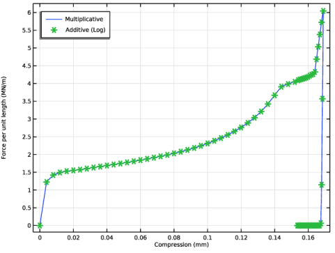
In the Settings window for Global, click Replace Expression in the upper-right corner of the y-Axis Data section. From the menu, choose Component 1 (comp1) > Definitions > Variables > reacF - Applied force from tool - N.
|
|
3
|
Locate the y-Axis Data section. In the table, enter the following settings:
|
|
4
|
|
5
|
|
6
|
|
1
|
|
2
|
|
3
|
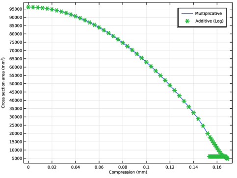
Locate the Plot Settings section. In the y-axis label text field, type Cross section area (mm<sup>2</sup>).
|
|
1
|
|
2
|
|
4
|
|
1
|
In the Model Builder window, under Component 1 (comp1) > Solid Mechanics (solid) click Linear Elastic Material 1.
|
|
2
|
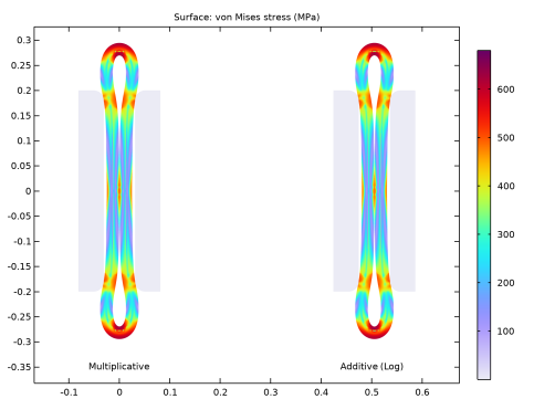
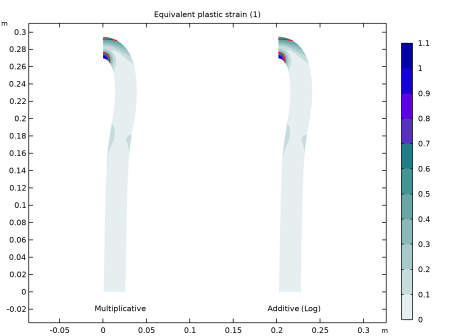
In the Settings window for Linear Elastic Material, type Linear Elastic Material: Multiplicative Decomposition in the Label text field.
|
|
1
|
In the Model Builder window, under Component 1 (comp1) > Solid Mechanics (solid) click Linear Elastic Material 2.
|
|
2
|
In the Settings window for Linear Elastic Material, type Linear Elastic Material: Additive Decomposition (Logarithmic) in the Label text field.
|
|
3
|
|
4
|
|
5
|
|
1
|
|
2
|
In the Settings window for Study, type Study 1: Multiplicative Decomposition in the Label text field.
|
|
1
|
|
2
|
|
3
|
Select the Modify model configuration for study step checkbox.
|
|
4
|
In the tree, select Component 1 (comp1) > Solid Mechanics (solid), Controls spatial frame > Linear Elastic Material: Additive Decomposition (Logarithmic).
|
|
5
|
Click
|
|
1
|
|
2
|
Go to the Add Study window.
|
|
3
|
|
4
|
Click the Add Study button in the window toolbar.
|
|
5
|
|
1
|
In the Settings window for Study, type Study 2: Additive Decomposition (Logarithmic) in the Label text field.
|
|
2
|
|
1
|
In the Model Builder window, under Study 2: Additive Decomposition (Logarithmic) click Step 1: Stationary.
|
|
2
|
|
3
|
Select the Auxiliary sweep checkbox.
|
|
4
|
Click
|
|
1
|
|
2
|
|
3
|
In the Model Builder window, expand the Study 2: Additive Decomposition (Logarithmic) > Solver Configurations > Solution 2 (sol2) > Stationary Solver 1 node, then click Parametric 1.
|
|
4
|
|
5
|
|
6
|
Select the Tuning of step size checkbox.
|
|
7
|
|
8
|
|
9
|
|
1
|
|
2
|
|
3
|
|
1
|
|
2
|
|
3
|
|
1
|
|
2
|
|
3
|
|
4
|
Clear the Parameter indicator text field.
|
|
5
|
|
6
|
|
7
|
|
8
|
|
1
|
In the Model Builder window, under Results > Stress (solid) right-click Surface 1 and choose Duplicate.
|
|
2
|
|
3
|
|
4
|
|
5
|
|
1
|
|
2
|
|
3
|
|
5
|
|
6
|
|
7
|
|
8
|
|
1
|
|
2
|
|
3
|
|
4
|
Clear the Parameter indicator text field.
|
|
5
|
|
6
|
|
7
|
|
1
|
|
2
|
|
3
|
Select the Manual indexing checkbox.
|
|
1
|
In the Model Builder window, under Results > Equivalent Plastic Strain (solid) right-click Surface 1 and choose Duplicate.
|
|
2
|
|
3
|
|
4
|
|
1
|
In the Model Builder window, under Results > Equivalent Plastic Strain (solid) right-click Contour 1 and choose Duplicate.
|
|
2
|
|
3
|
|
4
|
|
5
|
|
1
|
In the Model Builder window, right-click Equivalent Plastic Strain (solid) and choose Paste Table Annotation.
|
|
2
|
|
4
|
|
5
|
|
1
|
|
2
|
|
3
|
Select the Show legends checkbox.
|
|
4
|
|
1
|
|
2
|
|
3
|
|
4
|
Clear the Solution checkbox.
|
|
5
|
Clear the Description checkbox.
|
|
1
|
|
2
|
|
3
|
Locate the Data section. From the Dataset list, choose Study 2: Additive Decomposition (Logarithmic)/Solution 2 (sol2).
|
|
4
|
Click to expand the Coloring and Style section. Find the Line style subsection. From the Line list, choose None.
|
|
5
|
|
1
|
|
2
|
|
3
|
Select the Show legends checkbox.
|
|
1
|
|
2
|
|
3
|
|
4
|
Clear the Solution checkbox.
|
|
5
|
Clear the Description checkbox.
|
|
1
|
|
2
|
|
3
|
Locate the Data section. From the Dataset list, choose Study 2: Additive Decomposition (Logarithmic)/Solution 2 (sol2).
|
|
4
|
Locate the Coloring and Style section. Find the Line style subsection. From the Line list, choose None.
|
|
5
|
|
1
|
In the Model Builder window, under Results > Remaining Cross-Section Area right-click Global Evaluation 1 and choose Duplicate.
|
|
2
|
|
3
|
|
4
|
|
5
|