PDF

Powder Compaction of a Rotational Flanged Component
Introduction
The powder compaction process is common in the manufacturing industry, thanks to its potential to produce components of complex shape and high strength. Because the mechanical properties of the produced component depend on the final density, uniform densification is important. Large variations in density can make a part weak, which affects the overall quality of the component. Finite element analysis with a properly chosen constitutive material model is a handy tool that can provide detailed information about densification, punch forces, friction phenomena, plastic deformation, and internal stresses, in order to better understand the process and to improve the quality of the manufacturing process.
The constitutive material models that are relevant for this type of simulations can broadly be classified in two types:
1
2
This example studies the compaction of a rotational flanged component made of iron powder. As the porosity of the powder is large before compaction, a granular material model like the Capped Drucker–Prager (DPC) model is best suited as argued in Ref. 1 and Ref. 2. The elastic regime is represented by a linear elastic material, while a multiplicative plastic strain formulation together with a DPC yield function is used for the plastic regime. Additionally, friction between the powder and the die is taken into account. Simultaneous movement of the top and bottom punches is applied to avoid mesh distortion and other numerical problems. The simulation is performed using a 2D structured mesh with a linear displacement field as reported in Ref. 2.
Model Definition
The geometry of the workpiece (metal powder) and the die is shown in Figure 1. The punch that compacts the workpiece is not modeled. Instead, a prescribed displacement in the normal direction is used to compact the powder. Due to the axial symmetry, the size of model can be reduced.
Figure 1: Geometry of the workpiece (metal powder) and the die.
Material Properties
For the iron metal powder, an elastoplastic material model with a constitutive relation given by a combination of the linear elastic material model and the Capped Drucker–Prager (DPC) model is used. The material parameters are listed below.
The material of the die is assumed to be rigid. Therefore, it does no require any physics nor material properties.
Boundary Conditions
A prescribed displacement boundary condition is used for the upper and lower faces of the metal powder. The displacement in the z direction is controlled by an interpolation function.
Contact
The mesh on the source only needs to resolve the geometry of the contact surface. Hence no mesh is needed for the domain, but in order to show the die domains in the postprocessing plots the die domains are coarsely meshed.
Results and Discussion
Figure 2 shows the volumetric plastic strain at the end of the compaction process. At the middle corner, the compressive volumetric plastic strain is at its minimum, while it at the top corner is at its maximum.
The compaction process reduces the porosity of the iron powder and increases its density. This process also results in an increase in the strength of the component. Considering the type of geometry and loading, nonuniform changes in porosity are expected. Contours of the current relative density at the middle and at the end of the compaction are shown in Figure 3 and Figure 4, respectively. The metal powder in the thin lower portion of the workpiece is more compacted than the material in the middle or top portion. At the corners, the metal powder is less compacted due to the friction effects
Lastly, the von Mises stress along in the workpiece at the end of compaction is shown in Figure 5 in a 3D representation of the model.
Figure 2: Volumetric plastic strain at the end of compaction.
.
Figure 3: Current relative density in the middle of compaction.
Figure 4: Current relative density at the end of compaction.
Figure 5: Distribution of the von Mises stress in the workpiece at the end of the compaction process.
Notes About the COMSOL Implementation
The density distribution in the compaction process is affected by the contact pressure and the friction forces, so the accuracy of the contact algorithm is important in the powder compaction process. In this example, the Augmented Lagrangian method with a Fully Coupled solver is used.
References
1. A. Perez-Foguet, A. Rodriguez-Ferran, and A. Huerta, “Consistent tangent matrices for density-dependent finite plasticity models,” Int. J. Numer. Anal. Meth. Geomech., vol. 25, pp. 1045–1075, 2001.
2. A.R. Khoei, A. Shamloo, and A.R. Azami, “Extended finite element method in plasticity forming of powder compaction with contact friction,” Int.J. Solids Struct., vol. 43, pp. 5421–5448, 2006..
Application Library path: Nonlinear_Structural_Materials_Module/Porous_Plasticity/compaction_of_a_rotational_flange
Modeling Instructions
From the File menu, choose New.
New
In the New window, click  Model Wizard.
Model Wizard
1
In the Model Wizard window, click  2D Axisymmetric.
2
In the Select Physics tree, select Structural Mechanics > Solid Mechanics (solid).
3
Click Add.
4
Click  Study.
5
In the Select Study tree, select General Studies > Stationary.
6
Global Definitions
Parameters 1
1
In the Model Builder window, under Global Definitions click Parameters 1.
2
In the Settings window for Parameters, locate the Parameters section.
3
Definitions
Top Punch Displacement
1
In the Definitions toolbar, click  Interpolation.
2
In the Settings window for Interpolation, type Top Punch Displacement in the Label text field.
3
Locate the Definition section. In the Function name text field, type disp1.
4
5
Locate the Units section. In the Argument table, enter the following settings:
6
In the Function table, enter the following settings:
Bottom Punch Displacement
1
Right-click Top Punch Displacement and choose Duplicate.
2
In the Settings window for Interpolation, type Bottom Punch Displacement in the Label text field.
3
Locate the Definition section. In the table, enter the following settings:
Geometry 1
Rectangle 1 (r1)
1
In the Geometry toolbar, click  Rectangle.
2
In the Model Builder window, click Geometry 1.
3
In the Settings window for Geometry, locate the Units section.
4
From the Length unit list, choose mm.
5
In the Model Builder window, click Rectangle 1 (r1).
6
In the Settings window for Rectangle, locate the Size and Shape section.
7
In the Width text field, type 6.3.
8
In the Height text field, type 25.4.
9
Click  Build Selected.
Rectangle 2 (r2)
1
Right-click Rectangle 1 (r1) and choose Duplicate.
2
In the Settings window for Rectangle, locate the Size and Shape section.
3
In the Width text field, type 4.6.
4
In the Height text field, type 13.7.
5
Locate the Position section. In the r text field, type 6.3.
6
Click  Build Selected.
Rectangle 3 (r3)
1
Right-click Rectangle 2 (r2) and choose Duplicate.
2
In the Settings window for Rectangle, locate the Size and Shape section.
3
In the Width text field, type 20.2.
4
In the Height text field, type 11.7.
5
Locate the Position section. In the z text field, type 13.7.
6
Click  Build Selected.
Union 1 (uni1)
1
In the Geometry toolbar, click  Booleans and Partitions and choose Union.
2
Select the objects r2 and r3 only.
3
In the Settings window for Union, click  Build Selected.
Rectangle 4 (r4)
1
In the Model Builder window, under Component 1 (comp1) > Geometry 1 right-click Rectangle 3 (r3) and choose Duplicate.
2
In the Settings window for Rectangle, locate the Size and Shape section.
3
In the Width text field, type 15.6.
4
In the Height text field, type 13.7.
5
Locate the Position section. In the r text field, type 10.9.
6
In the z text field, type 0.
7
Click  Build Selected.
8
Click the  Zoom Extents button in the Graphics toolbar.
Rectangle 5 (r5)
1
Right-click Rectangle 4 (r4) and choose Duplicate.
2
In the Settings window for Rectangle, locate the Size and Shape section.
3
In the Width text field, type 6.3.
4
In the Height text field, type 25.4.
5
Locate the Position section. In the r text field, type 26.5.
6
Click  Build Selected.
Union 2 (uni2)
1
In the Geometry toolbar, click  Booleans and Partitions and choose Union.
2
Click the  Zoom Extents button in the Graphics toolbar.
3
Select the objects r4 and r5 only.
4
In the Settings window for Union, locate the Union section.
5
Clear the Keep interior boundaries checkbox.
6
Click  Build Selected.
Rectangle 1 (r1)
In the Model Builder window, under Component 1 (comp1) > Geometry 1 right-click Rectangle 1 (r1) and choose Group.
Internal Die
In the Settings window for Group, type Internal Die in the Label text field.
Rectangle 2 (r2), Rectangle 3 (r3), Union 1 (uni1)
1
In the Model Builder window, under Component 1 (comp1) > Geometry 1, Ctrl-click to select Rectangle 2 (r2), Rectangle 3 (r3), and Union 1 (uni1).
2
Compact
In the Settings window for Group, type Compact in the Label text field.
Rectangle 4 (r4), Rectangle 5 (r5), Union 2 (uni2)
1
In the Model Builder window, under Component 1 (comp1) > Geometry 1, Ctrl-click to select Rectangle 4 (r4), Rectangle 5 (r5), and Union 2 (uni2).
2
External Die
In the Settings window for Group, type External Die in the Label text field.
Form Union (fin)
1
In the Model Builder window, under Component 1 (comp1) > Geometry 1 click Form Union (fin).
2
In the Settings window for Form Union/Assembly, locate the Form Union/Assembly section.
3
From the Action list, choose Form an assembly.
4
From the Pair type list, choose Contact pair.
5
Click  Build Selected.
Add the interior edge in the workpiece geometry to Mesh Control Edges in order to generate a structured mesh.
Mesh Control Edges 1 (mce1)
1
In the Geometry toolbar, click  Virtual Operations and choose Mesh Control Edges.
2
On the object fin, select Boundary 8 only.
3
In the Settings window for Mesh Control Edges, click  Build Selected.
In subsequent steps, the side domain will be not be part of the physics. Hence use the toggle button in Contact Pair to switch the boundaries, so that the workpiece boundaries are chosen as destination boundaries.
Definitions
Contact Pair 2 (ap2)
1
In the Model Builder window, under Component 1 (comp1) > Definitions click Contact Pair 2 (ap2).
2
In the Settings window for Pair, click the  Swap Source and Destination button.
3
Locate the Source Boundaries section. Click to select the  Activate Selection toggle button.
4
Locate the Destination Boundaries section. Click to select the  Activate Selection toggle button.
Domains 1 and 3 (die) are considered as rigid and fixed, hence there is no need to consider them in physics, only a mesh is required.
Change the discretization to Linear.
Solid Mechanics (solid)
1
In the Model Builder window, under Component 1 (comp1) click Solid Mechanics (solid).
2
In the Settings window for Solid Mechanics, locate the Domain Selection section.
3
Click  Clear Selection.
4
5
Click to expand the Discretization section. From the Displacement field list, choose Linear.
For the elastoplastic analysis of the workpiece, choose a Capped DruckerPrager model by adding a Porous Plasticity subnode to the Linear Elastic Material. Set the formulation to Total Lagrangian to force large strains to be used.
Linear Elastic Material 1
1
In the Model Builder window, under Component 1 (comp1) > Solid Mechanics (solid) click Linear Elastic Material 1.
2
In the Settings window for Linear Elastic Material, locate the Geometric Nonlinearity section.
3
From the Formulation list, choose Total Lagrangian.
4
From the Strain decomposition list, choose Multiplicative.
Porous Plasticity 1
1
In the Physics toolbar, click  Attributes and choose Porous Plasticity.
2
In the Settings window for Porous Plasticity, locate the Porous Plasticity Model section.
3
From the Material model list, choose Capped Drucker–Prager.
4
Locate the Cap Model section. From the Hardening model list, choose Exponential.
For better accuracy, select the Augmented Lagrangian with a Fully Coupled solution method.
Contact 1
1
In the Model Builder window, under Component 1 (comp1) > Solid Mechanics (solid) click Contact 1.
2
In the Settings window for Contact, locate the Contact Method section.
3
From the list, choose Augmented Lagrangian.
4
From the Solution method list, choose Fully coupled.
Friction 1
1
In the Physics toolbar, click  Attributes and choose Friction.
2
In the Settings window for Friction, locate the Friction Parameters section.
3
In the μ text field, type 0.08.
Prescribed Displacement 1
1
In the Physics toolbar, click  Boundaries and choose Prescribed Displacement.
2
3
In the Settings window for Prescribed Displacement, locate the Prescribed Displacement section.
4
From the Displacement in z direction list, choose Prescribed.
5
In the u0z text field, type disp1(t).
Prescribed Displacement 2
1
In the Physics toolbar, click  Boundaries and choose Prescribed Displacement.
2
3
In the Settings window for Prescribed Displacement, locate the Prescribed Displacement section.
4
From the Displacement in z direction list, choose Prescribed.
5
In the u0z text field, type disp2(t).
Materials
Iron Powder
1
In the Model Builder window, under Component 1 (comp1) right-click Materials and choose Blank Material.
2
In the Settings window for Material, type Iron Powder in the Label text field.
3
4
Locate the Material Contents section. In the table, enter the following settings:
Mesh 1
Mapped 1
1
In the Mesh toolbar, click  Mapped.
2
In the Settings window for Mapped, locate the Domain Selection section.
3
From the Geometric entity level list, choose Domain.
4
5
Click to expand the Control Entities section. From the Smooth across removed control entities list, choose Off.
6
Click to expand the Reduce Element Skewness section. Select the Adjust edge mesh checkbox.
Distribution 1
1
Right-click Mapped 1 and choose Distribution.
2
3
In the Settings window for Distribution, locate the Distribution section.
4
In the Number of elements text field, type 4.
Distribution 2
1
In the Model Builder window, right-click Mapped 1 and choose Distribution.
2
3
In the Settings window for Distribution, locate the Distribution section.
4
In the Number of elements text field, type 20.
Mapped 2
1
In the Mesh toolbar, click  Mapped.
2
In the Settings window for Mapped, locate the Domain Selection section.
3
From the Geometric entity level list, choose Domain.
4
5
Locate the Control Entities section. From the Smooth across removed control entities list, choose Off.
6
Locate the Reduce Element Skewness section. Select the Adjust edge mesh checkbox.
Distribution 1
1
Right-click Mapped 2 and choose Distribution.
2
3
In the Settings window for Distribution, locate the Distribution section.
4
In the Number of elements text field, type 20.
Distribution 2
1
In the Model Builder window, right-click Mapped 2 and choose Distribution.
2
3
In the Settings window for Distribution, locate the Distribution section.
4
In the Number of elements text field, type 16.
Size
1
In the Model Builder window, under Component 1 (comp1) > Mesh 1 click Size.
2
In the Settings window for Size, locate the Element Size section.
3
From the Predefined list, choose Coarser.
Free Quad 1
1
In the Mesh toolbar, click  Free Quad.
2
In the Settings window for Free Quad, click  Build All.
Augmented Lagrangian contact in addition to the material and geometric nonlinearity in the model demands special solver settings to achieve smooth convergence.
Study 1
Step 1: Stationary
Set up an auxiliary continuation sweep for the t parameter.
1
In the Model Builder window, under Study 1 click Step 1: Stationary.
2
In the Settings window for Stationary, click to expand the Study Extensions section.
3
Select the Auxiliary sweep checkbox.
4
5
Solution 1 (sol1)
1
In the Study toolbar, click  Show Default Solver.
2
In the Model Builder window, expand the Solution 1 (sol1) node.
Set up the solver in order to improve the convergence.
3
In the Model Builder window, expand the Study 1 > Solver Configurations > Solution 1 (sol1) > Stationary Solver 1 node, then click Parametric 1.
4
In the Settings window for Parametric, click to expand the Continuation section.
5
Select the Tuning of step size checkbox.
6
In the Minimum step size text field, type 0.0005.
7
In the Maximum step size text field, type 0.2.
8
From the Predictor list, choose Linear.
9
In the Model Builder window, under Study 1 > Solver Configurations > Solution 1 (sol1) > Stationary Solver 1 click Fully Coupled 1.
10
In the Settings window for Fully Coupled, click to expand the Method and Termination section.
11
From the Nonlinear method list, choose Automatic (Newton).
12
In the Study toolbar, click  Compute.
Result Templates
1
In the Results toolbar, click  Result Templates to open the Result Templates window.
2
Go to the Result Templates window.
3
In the tree, select Study 1/Solution 1 (sol1) > Solid Mechanics > Volumetric Plastic Strain (solid) and Study 1/Solution 1 (sol1) > Solid Mechanics > Current Void Volume Fraction (solid).
4
Click the Add Result Template button in the window toolbar.
5
In the Results toolbar, click  Result Templates to close the Result Templates window.
Results
Study 1/Solution 1 (sol1)
In the Model Builder window, expand the Results > Datasets node, then click Study 1/Solution 1 (sol1).
Selection
1
In the Results toolbar, click  Attributes and choose Selection.
2
In the Settings window for Selection, locate the Geometric Entity Selection section.
3
From the Geometric entity level list, choose Domain.
4
In order to visualize the von Mises stress in the deformed workpiece along with the undeformed dies, duplicate the Study 1/Solution 1 dataset, and set the selection to domains 1 and 3. Set up a new Revolution 2D dataset based on Study 1/Solution 1 (2).
Study 1/Solution 1 (2) (sol1)
Right-click Study 1/Solution 1 (sol1) and choose Duplicate.
Selection
1
In the Model Builder window, expand the Study 1/Solution 1 (2) (sol1) node, then click Selection.
2
In the Settings window for Selection, locate the Geometric Entity Selection section.
3
Click  Clear Selection.
4
Revolution 2D 1
1
In the Model Builder window, right-click Revolution 2D and choose Duplicate.
2
In the Settings window for Revolution 2D, locate the Data section.
3
From the Dataset list, choose Study 1/Solution 1 (2) (sol1).
In order to visualize the undeformed dies, set up Surface 2 node in the next 3D plot with a zero expression. Select the Revolution 2D 2 dataset, and add a Material Appearance node for the visualization.
Stress, 3D (solid)
1
In the Model Builder window, expand the Results > Stress, 3D (solid) node, then click Stress, 3D (solid).
2
In the Settings window for 3D Plot Group, locate the Plot Settings section.
3
Clear the Plot dataset edges checkbox.
Surface 2
1
Right-click Stress, 3D (solid) and choose Surface.
2
In the Settings window for Surface, locate the Data section.
3
From the Dataset list, choose Revolution 2D 1.
4
Locate the Expression section. In the Expression text field, type 0.
5
Click to expand the Title section. From the Title type list, choose None.
Material Appearance 1
1
Right-click Surface 2 and choose Material Appearance.
2
In the Settings window for Material Appearance, locate the Appearance section.
3
From the Appearance list, choose Custom.
4
From the Material type list, choose Steel.
5
In the Stress, 3D (solid) toolbar, click  Plot.
Volumetric Plastic Strain (solid)
1
In the Model Builder window, under Results click Volumetric Plastic Strain (solid).
2
In the Settings window for 2D Plot Group, click to expand the Number Format section.
3
Select the Manual color legend settings checkbox.
4
In the Precision text field, type 4.
Surface 1
1
In the Model Builder window, expand the Volumetric Plastic Strain (solid) node, then click Surface 1.
2
In the Settings window for Surface, locate the Coloring and Style section.
3
In the Number of bands text field, type 6.
Deformation 1
1
Right-click Surface 1 and choose Deformation.
2
In the Settings window for Deformation, locate the Scale section.
3
Select the Scale factor checkbox. In the associated text field, type 1.
4
In the Volumetric Plastic Strain (solid) toolbar, click  Plot.
Current Relative Density at Middle of Compaction
1
In the Model Builder window, under Results click Current Void Volume Fraction (solid).
2
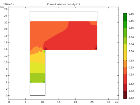
In the Settings window for 2D Plot Group, type Current Relative Density at Middle of Compaction in the Label text field.
3
Locate the Data section. From the Parameter value (t (s)) list, choose 5.
Surface 1
1
In the Model Builder window, expand the Current Relative Density at Middle of Compaction node, then click Surface 1.
2
In the Settings window for Surface, click Replace Expression in the upper-right corner of the Expression section. From the menu, choose Component 1 (comp1) > Solid Mechanics > Porous plasticity > solid.rhorelGp - Current relative density - 1.
3
Locate the Expression section. Clear the Description checkbox.
4
Locate the Coloring and Style section. From the Color table transformation list, choose Reverse.
5
In the Current Relative Density at Middle of Compaction toolbar, click  Plot.
Current Relative Density at End of Compaction
1
In the Model Builder window, right-click Current Relative Density at Middle of Compaction and choose Duplicate.
2
In the Settings window for 2D Plot Group, type Current Relative Density at End of Compaction in the Label text field.
3
Locate the Data section. From the Parameter value (t (s)) list, choose 10.
4
In the Current Relative Density at End of Compaction toolbar, click  Plot.