|
|
|


|
1
|
|
2
|
In the Select Physics tree, select Structural Mechanics > Explicit Dynamics > Solid Mechanics, Explicit Dynamics (solid).
|
|
3
|
Click Add.
|
|
4
|
Click
|
|
5
|
In the Select Study tree, select Preset Studies for Selected Physics Interfaces > Explicit Dynamics.
|
|
6
|
Click
|
|
1
|
|
2
|
|
3
|
|
4
|
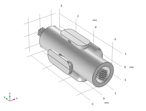
Browse to the model’s Application Libraries folder and double-click the file cable_crimping_parameters.txt.
|
|
1
|
|
2
|
|
3
|
|
4
|
|
5
|
|
6
|
|
1
|
|
2
|
Browse to the model’s Application Libraries folder and double-click the file cable_crimping_geom_sequence.mph.
|
|
3
|
|
4
|
|
5
|
|
1
|
In the Model Builder window, under Component 1 (comp1) click Solid Mechanics, Explicit Dynamics (solid).
|
|
2
|
In the Settings window for Solid Mechanics, Explicit Dynamics, click to expand the Energy Dissipation section.
|
|
3
|
|
1
|
In the Model Builder window, under Component 1 (comp1) > Solid Mechanics, Explicit Dynamics (solid) click Linear Elastic Material 1.
|
|
2
|
|
3
|
|
4
|
|
1
|
|
2
|
|
3
|
From the Selection list, choose Deformable Domains to model only the terminal and the wires as elastoplastic materials.
|
|
1
|
|
2
|
|
3
|
|
4
|
|
1
|
|
2
|
|
3
|
|
1
|
|
1
|
|
3
|
|
4
|
|
1
|
|
3
|
|
4
|
|
1
|
|
3
|
|
4
|
|
1
|
|
3
|
|
4
|
|
1
|
In the Model Builder window, under Component 1 (comp1) right-click Materials and choose Blank Material.
|
|
2
|
|
3
|
|
4
|
|
5
|
Locate the Material Contents section. In the table, enter the following settings:
|
|
1
|
|
2
|
|
3
|
|
4
|
Locate the Material Contents section. In the table, enter the following settings:
|
|
1
|
|
2
|
|
3
|
|
4
|
Locate the Material Contents section. In the table, enter the following settings:
|
|
1
|
|
1
|
|
3
|
|
4
|
Click to select the
|
|
5
|
|
6
|
|
1
|
|
2
|
|
3
|
Click the Custom button.
|
|
4
|
|
5
|
|
1
|
|
2
|
|
3
|
|
4
|
|
5
|
Click
|
|
1
|
|
1
|
|
3
|
|
4
|
|
1
|
|
2
|
|
3
|
|
4
|
|
1
|
|
2
|
|
3
|
|
4
|
In the Relative placement of vertices along edge text field, type range(0,0.1,1) range(1.05,0.05,2) range(2.1,0.1,3).
|
|
5
|
Click
|
|
1
|
|
1
|
|
2
|
|
3
|
Click the Custom button.
|
|
4
|
Locate the Element Size Parameters section.
|
|
5
|
|
1
|
|
2
|
|
3
|
|
4
|
Click
|
|
1
|
|
2
|
|
3
|
|
4
|
|
5
|
|
1
|
|
2
|
|
3
|
|
4
|
|
5
|
Click
|
|
1
|
|
2
|
|
3
|
Click
|
|
4
|
|
5
|
|
6
|
Click OK.
|
|
7
|
|
9
|
Click
|
|
1
|
|
2
|
|
3
|
|
1
|
|
2
|
|
3
|
|
4
|
|
5
|
|
6
|
|
1
|
|
2
|
|
3
|
|
4
|
|
1
|
|
2
|
|
3
|
Select the Plot checkbox.
|
|
5
|
|
1
|
|
2
|
Clear the Plot dataset edges checkbox.
|
|
3
|
Click
|
|
1
|
|
2
|
|
3
|
|
4
|
|
5
|
|
6
|
|
7
|
|
8
|
Clear the Color checkbox.
|
|
9
|
Clear the Color and data range checkbox.
|
|
1
|
|
2
|
|
3
|
|
4
|
|
1
|
|
2
|
|
3
|
|
1
|
|
2
|
|
3
|
|
1
|
|
2
|
|
3
|
|
4
|
|
1
|
|
2
|
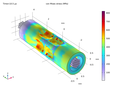
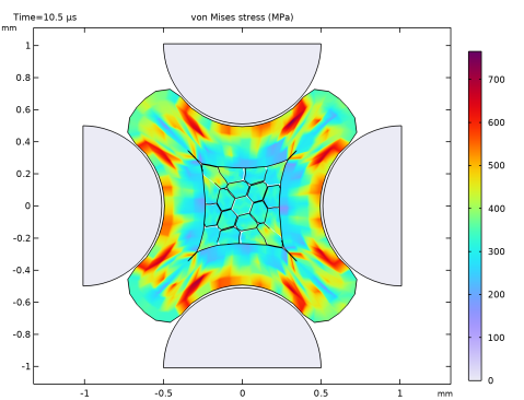
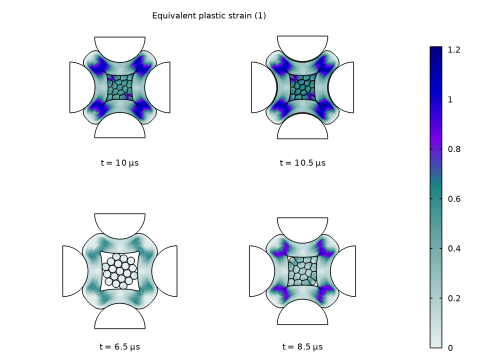
In the Settings window for 2D Plot Group, type Equivalent Plastic Strain, Cross Section in the Label text field.
|
|
3
|
|
4
|
|
5
|
|
6
|
|
7
|
Click to collapse the Title section. Locate the Plot Settings section. From the View list, choose New view.
|
|
8
|
|
1
|
In the Model Builder window, expand the Equivalent Plastic Strain, Cross Section node, then click Surface 1.
|
|
2
|
|
3
|
|
4
|
|
1
|
|
2
|
|
3
|
|
4
|
|
5
|
|
6
|
|
7
|
|
8
|
Clear the Color checkbox.
|
|
9
|
Clear the Color and data range checkbox.
|
|
10
|
|
1
|
In the Model Builder window, right-click Equivalent Plastic Strain, Cross Section and choose Annotation.
|
|
2
|
|
3
|
|
4
|
|
5
|
|
6
|
|
7
|
|
8
|
|
1
|
|
2
|
|
3
|
|
4
|
|
5
|
|
1
|
|
2
|
|
3
|
|
4
|
|
1
|
|
2
|
|
3
|
|
4
|
|
5
|
|
1
|
|
2
|
|
3
|
|
4
|
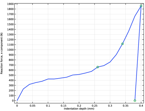
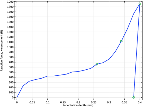
Click Add Expression in the upper-right corner of the y-Axis Data section. From the menu, choose Component 1 (comp1) > Solid Mechanics, Explicit Dynamics > Reactions > Prescribed Displacement 1 > Reaction force (spatial frame) - N > solid.pdisp1.RFsumx - Reaction force, x-component.
|
|
5
|
|
6
|
|
7
|
|
8
|
|
1
|
|
2
|
|
3
|
|
4
|
Locate the Coloring and Style section. Find the Line style subsection. From the Line list, choose None.
|
|
5
|
|
6
|
|
1
|
|
2
|
|
1
|
|
2
|
|
1
|
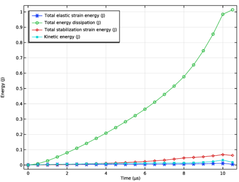
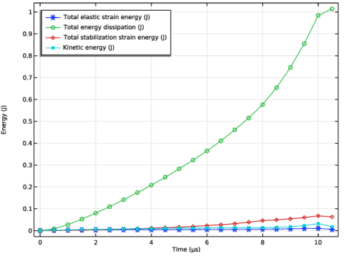
In the Model Builder window, right-click Energy Evaluation and choose Integration > Volume Integration.
|
|
2
|
|
3
|
|
4
|
Locate the Expressions section. In the table, enter the following settings:
|
|
5
|
Locate the Integration Settings section.
|
|
6
|
|
7
|
|
1
|
Go to the Energy Evaluation window.
|
|
2
|
Click the Table Graph button in the window toolbar.
|
|
1
|
|
2
|
|
3
|
|
1
|
|
2
|
|
3
|
Locate the Plot Settings section.
|
|
4
|
|
5
|
|
6
|
|
1
|
|
2
|
Click
|
|
1
|
|
2
|
|
3
|
|
4
|
Browse to the model’s Application Libraries folder and double-click the file cable_crimping_parameters.txt.
|
|
1
|
|
2
|
|
3
|
|
1
|
|
2
|
|
3
|
|
4
|
|
1
|
|
2
|
|
3
|
|
1
|
Right-click Component 1 (comp1) > Geometry 1 > Work Plane 1 (wp1) > Plane Geometry > Circle 1 (c1) and choose Duplicate.
|
|
2
|
|
3
|
|
1
|
|
2
|
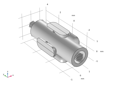
Select the object c2 only.
|
|
3
|
|
4
|
|
1
|
|
2
|
|
3
|
|
4
|
|
1
|
|
2
|
|
3
|
|
4
|
|
1
|
|
2
|
|
3
|
|
4
|
|
5
|
|
6
|
|
7
|
|
1
|
|
2
|
On the object wp1, select Boundaries 1–19 only.
|
|
3
|
|
4
|
|
5
|
On the object ls1, select Edge 1 only.
|
|
6
|
Locate the Motion of Cross Section section. Find the Additional twisting and scaling subsection. In the Twist angle text field, type theta*s.
|
|
7
|
Click
|
|
1
|
|
2
|
|
3
|
|
4
|
|
5
|
|
6
|
|
7
|
Click to expand the Layers section. In the table, enter the following settings:
|
|
1
|
|
2
|
|
3
|
|
4
|
On the object cyl1, select Domain 3 only.
|
|
1
|
|
2
|
|
3
|
|
1
|
|
2
|
|
3
|
|
4
|
Locate the Coordinates section. In the table, enter the following settings:
|
|
1
|
|
2
|
|
3
|
|
4
|
|
5
|
|
6
|
|
7
|
|
8
|
|
9
|
|
1
|
|
2
|
|
3
|
|
4
|
Locate the Coordinates section. In the table, enter the following settings:
|
|
1
|
|
2
|
Click in the Graphics window and then press Ctrl+A to select all objects.
|
|
3
|
|
4
|
Select the Keep input objects checkbox.
|
|
5
|
|
6
|
|
1
|
|
2
|
Click in the Graphics window and then press Ctrl+A to select all objects.
|
|
1
|
|
2
|
|
3
|
Click the Angles button.
|
|
4
|
|
5
|
|
1
|
|
2
|
|
3
|
|
1
|
|
2
|
|
3
|
|
4
|
|
5
|
|
6
|
|
1
|
Right-click Component 1 (comp1) > Geometry 1 > Work Plane 3 (wp3) > Plane Geometry > Circular Arc 1 (ca1) and choose Duplicate.
|
|
2
|
|
3
|
|
4
|
|
5
|
|
6
|
|
1
|
|
2
|
|
3
|
|
4
|
Locate the Coordinates section. In the table, enter the following settings:
|
|
1
|
|
2
|
Click in the Graphics window and then press Ctrl+A to select all objects.
|
|
3
|
|
4
|
Select the Keep input objects checkbox.
|
|
5
|
|
6
|
|
1
|
|
2
|
Click in the Graphics window and then press Ctrl+A to select all objects.
|
|
1
|
|
2
|
|
1
|
|
2
|
Select the object rev1 only.
|
|
3
|
|
4
|
|
5
|
Select the object ext1 only.
|
|
6
|
Click
|
|
1
|
|
2
|
|
3
|
|
4
|
On the object dif1, select Boundary 3 only.
|
|
5
|
Select the Group by continuous tangent checkbox.
|
|
1
|
|
2
|
|
3
|
|
4
|
On the object dif1, select Boundary 17 only.
|
|
5
|
Select the Group by continuous tangent checkbox.
|
|
1
|
|
2
|
Select the object dif1 only.
|
|
3
|
|
4
|
|
5
|
|
1
|
|
2
|
|
3
|
|
4
|
Clear the Create pairs checkbox.
|
|
5
|
|
1
|
|
2
|
On the object fin, select Domains 2–5 only.
|
|
1
|
|
2
|
|
3
|
|
1
|
|
2
|
|
3
|
|
4
|
|
5
|
|
1
|
|
2
|
|
3
|
On the object cmf2, select Domains 5–23 only.
|
|
1
|
|
2
|
|
3
|
On the object cmf2, select Domain 2 only.
|
|
1
|
|
2
|
|
3
|
On the object cmf2, select Domains 1, 3, 4, and 24 only.
|
|
1
|
|
2
|
|
3
|
|
4
|
|
5
|
Click OK.
|
|
6
|