COMSOL 6.4 - Buckling of HDPE Liners

High Density Polyethylene (HDPE) is a thermoplastic material used in the oil and gas industry to make liners for damaged pipes, mainly due to its availability, low production costs, and ease of installation. These components have been reported to experience sudden collapse during idle times connected to maintenance, when the pressure inside the pipe drops. This type of failure is mainly caused by permeation of oil-derived gases between the liners and the inner pipe wall; the larger the volume of gas trapped in such a gap, the higher the pressure on the external surface of the liner, which will then lead to buckling when not balanced by pressure on the inner surface (Ref. 1).

The Bergstrom–Bischoff viscoplastic model has been shown to be suitable to predict the behavior of thermoplastic materials and can be used to foresee the collapse of HDPE liners under different working temperatures and loading strain rates.

Model Definition

This model uses a plane-strain approximation to simulate a 1 m long HDPE liner. The geometry of the cross section is depicted in Figure 1. The thickness of the liner is 6.2 mm and the nominal outer diameter is 114 mm. A small geometrical defect is introduced in order to facilitate convergence to a single-lobe buckling collapse, which is the one mostly reported experimentally. In particular, one diameter is made 0.2% shorter. Considering such a defected geometry, the problem shows one mirror symmetry along the short diameter. As a consequence, the computational cost can be reduced by modeling only half of the cross section and using symmetry boundary conditions. The pipe is modeled as an infinitely rigid body.

Figure 1: Model geometry.

Material Model

The inner surface of the liner is subjected to atmospheric pressure, simulating depressurization during shutdowns. The interaction between the gas in the annulus gap between the host pipe and the liner is instead simplified by the use of the ideal gas law, that is, the pressure acting on the outside of the liner is computed as

Here, T is the absolute working temperature, R is the gas constant, and M is the molar mass of the considered gas. The pressure loading the liner is increased by imposing a constant inflow mass rate:

Moreover, V is the current volume of the gap between the pipe and the liner, computed by accounting for the deformation of the liner.

The rheology of the Bergstrom–Bischoff material model is shown in Figure 2. It features a so-called equilibrium network that can be schematized as a simple hyperelastic spring characterized by an Arruda–Boyce strain energy, with a temperature-dependent shear modulus:

where θ0 and θr are material properties. Such an equilibrium network is placed in parallel with two other networks that model the nonequilibrium behavior. Each of the latter networks are defined by an isochoric Arruda–Boyce spring in series with a viscoplastic element whose rate multiplier is given by

(1)

where σvm is the von Mises stress of the nonequilibrium network and A, ai, ni, m, and σres,i identify material properties. The shear modulus of the nonequilibrium networks is controlled with an energy factor βvi that sets the relative stiffness of each nonequilibrium network with respect to the equilibrium one. The energy factor of the second nonequilibrium network is made dependent on the viscoplastic strain of the first one by the differential equation

where α and βv,f are material properties.

The numerical values of the material properties used in the model are given in Table 1, and are inspired by those found in Ref. 2.

Table 1: material properties.
Constant	Value	Description
μ0	9.25 MPa	Shear modulus
Nseg	4.5	Number of segments
ρ	950 kg/m3	Density
K	2 GPa	Bulk modulus
βv1	20	Energy factor, network 1
σres,1	7.1 MPa	Flow resistance, network 1
a	0.183	Pressure coefficient
n1	13	Stress exponent, network 1
βv,i	23.7	Initial energy factor, network 2
βv,f	11.2	Final energy factor, network 2
σres,2	32.2 MPa	Flow resistance, network 2
n2	22.4	Stress exponent
α	30	Energy factor evolution coefficient
θr	-94 K	Stiffness temperature response
m	117.2	Temperature exponent
θ0	273.15 K	Reference temperature

Figure 2: Rheology of the Bergstrom–Bischoff material model.

Results and Discussion

Figure 3 depicts the deformed shape of the liner after buckling at 278.15 K, showing the one-lobe type of collapse. The evolution of the gas pressure in the gap as a function of time is depicted in Figure 4, where it can be observed how the pressure suddenly drops after collapse as a consequence of the increased gap volume. The figure also shows how the collapse pressure reduces at high working temperatures.

Figure 3: One-lobe failure of the HDPE liner.

Figure 4: Evolution of pressure of the gas trapped in the gap between liner and pipe.

Notes About the COMSOL Implementation

•

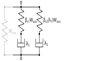
You can use the Bergstrom–Bischoff material model by adding a node under . Select in the section to add the temperature dependency to the rate multiplier. You find the option in the section under the node. This option can be faster than when the number of degrees of freedom is small.

•

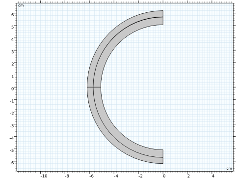
Add nodes to compute the volume inside the liner, as well as the volume formed in between the pipe and liner. The pipe boundaries forming the pipe–liner cavity are not included in the interface, but these external boundaries can still be included in .

•

Note that because of the intrinsic time-dependent nature of the Bergstrom–Bischoff model, the buckling analysis must be conducted in the time domain, retaining the inertial terms. In such a way, when the stiffness of the system becomes singular, the whole strain energy can be converted into kinetic energy.

•

The gas is assumed to permeate along the whole circumference of the liner in a uniform manner. For this reason, the pressure would be applied on the whole external surface of the liner, even if the initial nominal geometry assumes no gap between liner and pipe. To do that, select the option instead of the default under the section in the boundary condition. This section is visible when you select in the menu.

•

Add a study step before the one in order to compute consistent initial conditions, making contact easier to initiate at the first time steps. Use the stiffness of the Bergstrom–Bischoff material in the step.

References

1. F. Rueda, J.P. Torres, M. Machado, P.M. Frontini, and J.L. Otegui, “External pressure induced buckling collapse of high density polyethylene (HDPE) liners: FEM modeling and predictions,” Thin-Walled Struct., vol. 96, pp. 56–63, 2015.

2. F. Rueda, A. Marquez, J.L. Otegui, and P.M. Frontini, “Buckling collapse of HDPE liners: Experimental set-up and FEM simulations,” Thin-Walled Struct., vol. 109, pp. 103–112, 2016.

Nonlinear_Structural_Materials_Module/Viscoplasticity/buckling_hdpe_liner

Modeling Instructions

From the menu, choose .

New

In the window, click

Model Wizard

In the window, click

In the tree, select > .

Click .

Click

In the tree, select > .

Click

Global Definitions

Material Properties

In the window, under click .

In the window for , type Material Properties in the text field.

Locate the section. In the table, enter the following settings:


Name	Expression	Value	Description
mu	9.25[MPa]	9.25E6 Pa	Shear modulus
beta1	20	20	Energy factor, network 1
beta2_i	23.7	23.7	Initial energy factor, network 2
beta2_f	11.2	11.2	Final energy factor, network 2
alpha	30	30	Energy factor evolution coefficient
thetar	-94[K]	-94 K	Stiffness temperature response
m	117.2	117.2	Temperature exponent
theta0	273.15[K]	273.15 K	Reference temperature
T	293.15[K]	293.15 K	Temperature

Geometrical Parameters

In the toolbar, click

and choose > .

In the window for , type Geometrical Parameters in the text field.

Locate the section. In the table, enter the following settings:


Name	Expression	Value	Description
L	1[m]	1 m	Length of pipe
outer_r	114[mm]/2	0.057 m	Outer radius of liner
th_liner	6.2[mm]	0.0062 m	Thickness of liner
th_pipe	5[mm]	0.005 m	Thickness of pipe

Gas Properties

In the toolbar, click

and choose > .

In the window for , type Gas Properties in the text field.

Locate the section. In the table, enter the following settings:


Name	Expression	Value	Description
M	16.04[g/mol]	0.01604 kg/mol	Molar mass
Rs	R_const/M	518.36 J/(kg·K)	Gas constant per unit mass
mdot	750[cm^3/min]*0.657[kg/m^3]	8.2125E-6 kg/s	Mass flow rate

Geometry 1

In the window, under click .

In the window for , locate the section.

From the list, choose .

Circle 1 (c1)

In the toolbar, click

In the window for , locate the section.

In the text field, type outer_r.

In the text field, type 180.

Locate the section. In the text field, type 180.

Click to expand the section. In the table, enter the following settings:


Layer name	Thickness (cm)
Layer 1	th_liner

Click

Ellipse 1 (e1)

In the toolbar, click

In the window for , locate the section.

In the text field, type outer_r.

In the text field, type outer_r*0.996.

In the text field, type 180.

Click to expand the section. In the table, enter the following settings:


Layer name	Thickness (cm)
Layer 1	th_liner

Click

Delete Entities 1 (del1)

In the window, right-click and choose .

In the window for , locate the section.

From the list, choose .

On the object , select Domains 1 and 2 only.

On the object , select Domains 2 and 3 only.

Circle 2 (c2)

In the toolbar, click

In the window for , locate the section.

In the text field, type outer_r+th_pipe.

In the text field, type 180.

Locate the section. In the text field, type 90.

Click to expand the section. In the table, enter the following settings:


Layer name	Thickness (cm)
Layer 1	th_pipe

Click

Delete Entities 2 (del2)

Right-click and choose .

In the window for , locate the section.

From the list, choose .

On the object , select Domain 2 only.

Click

Click the

button in the toolbar.

Union 1 (uni1)

In the toolbar, click

and choose .

Select the objects and only.

In the window for , click

Form Union (fin)

In the window, under > click .

In the window for , locate the section.

From the list, choose .

Clear the checkbox.

In the toolbar, click

Definitions

Contact Pair 1 (p1)

In the toolbar, click

and choose .

Select Boundaries 6 and 7 only.

In the window for , locate the section.

Click

In the dialog, type Pipe Inner Surface in the text field.

Click .

In the window for , locate the section.

Click to select the

toggle button.

Select Boundaries 11 and 12 only.

Click

In the dialog, type Liner Outer Surface in the text field.

Click .

Liner Inner Surface

In the toolbar, click

In the window for , locate the section.

From the list, choose .

Select Boundaries 13 and 14 only.

In the text field, type Liner Inner Surface.

Pipe–Liner Cavity

In the toolbar, click

In the window for , locate the section.

From the list, choose .

Locate the section. Under , click

In the dialog, in the list, choose and .

Click .

In the window for , type Pipe-Liner Cavity in the text field.

You can include only the liner in , since the pipe is modeled as a rigid boundary.

Solid Mechanics (solid)

In the window, under click .

Select Domains 3 and 4 only.

In the window for , locate the section.

Click

In the dialog, type Liner in the text field.

Click .

In the window for , locate the section.

In the d text field, type L.

Contact 1

In the window, under > click .

In the window for , locate the section.

From the list, choose .

In the fp text field, type 8.

Symmetry 1

In the toolbar, click

and choose .

Select Boundaries 9 and 10 only.

Enclosed Cavity, Inner Pressure

In the toolbar, click

and choose .

In the window for , type Enclosed Cavity, Inner Pressure in the text field.

Locate the section. From the list, choose .

Locate the section. Click to select the

toggle button.

Select Point 11 only.

Locate the section. In the fV text field, type 2.

Remove the node, and use a node instead to apply a known pressure load on the liner’s inner boundary.

Fluid 1

In the window, right-click and choose .

Prescribed Pressure 1

In the toolbar, click

and choose .

In the window for , locate the section.

In the p text field, type 1[atm].

Next, model the cavity formed between the pipe and liner.

Enclosed Cavity, Outer Pressure

In the window, right-click and choose .

In the window for , type Enclosed Cavity, Outer Pressure in the text field.

Select the – to define the volume in between the pipe and liner. Notice that the pipe boundaries, which are not included in the interface, will be marked as "not applicable". These boundaries have to be explicitly allowed.

Locate the section. From the list, choose .

Click to expand the section. Select the checkbox.

When including external boundaries, a normal direction has to be specified. By convention, the normal for external boundaries has to point toward the fluid. In this case, the normal of the referenced default boundary system is oriented correctly.

Prescribed Pressure 1

In the window, expand the node, then click .

In the window for , locate the section.

In the p text field, type Rs*mdot*t*T/solid.enc2.V.

Hyperelastic Material 1

In the toolbar, click

and choose .

In the window for , locate the section.

From the list, choose .

Locate the section. From the list, choose .

From the list, choose .

Polymer Viscoplasticity 1

In the toolbar, click

and choose .

In the window for , locate the section.

From the list, choose .

Find the subsection. In the βv1 text field, type beta1.

Find the subsection. In the βv,i text field, type beta2_i.

In the βv,f text field, type beta2_f.

In the α text field, type alpha.

Locate the section. From the g(T) list, choose .

In the m text field, type m.

Locate the section. From the T list, choose . In the associated text field, type T.

Locate the section. In the Tref text field, type theta0.

Locate the section. From the list, choose .

Materials

HDPE

In the window, under right-click and choose .

In the window for , locate the section.

From the list, choose .

Locate the section. In the table, enter the following settings:


Property	Variable	Value	Unit	Property group
Bulk modulus	K	2[GPa]	N/m²	Bulk modulus and shear modulus
Number of segments	Nseg	4.5	1	Arruda-Boyce
Macroscopic shear modulus	mu0	mu*(1+(T-theta0)/thetar)	N/m²	Arruda-Boyce
Density	rho	950[kg/m^3]	kg/m³	Basic
Viscoplastic rate coefficient	A_BeBi	sqrt(2/3)[1/s]	1/s	Bergstrom-Bischoff viscoplasticity
Flow resistance	sigRes1_BeBi	7.1[MPa]	N/m²	Bergstrom-Bischoff viscoplasticity
Stress exponent	n1_BeBi	13	1	Bergstrom-Bischoff viscoplasticity
Pressure hardening coefficient	a1_BeBi	0.183	1	Bergstrom-Bischoff viscoplasticity
Flow resistance	sigRes2_BeBi	32.2[MPa]	N/m²	Bergstrom-Bischoff viscoplasticity
Stress exponent	n2_BeBi	22.4	1	Bergstrom-Bischoff viscoplasticity
Pressure hardening coefficient	a2_BeBi	0.183	1	Bergstrom-Bischoff viscoplasticity