COMSOL 6.4 - Biventricular Cardiac Model

This example demonstrates how to simulate a cardiac contraction on a simplified heart geometry, where only the ventricles are considered and the stimulus starts from the atrioventricular node.

During the cardiac cycle (heartbeat) an electrical stimulus generated from the sino–atrial node propagates throughout the entire heart. When excited, cardiac cells are subjected to an electric potential jump across their membranes. The transport and accumulation of ions and additional chemical reactions cause cells to contract. At a macroscale these chemical and electrical processes trigger the contraction of the muscle tissue, the myocardium, allowing blood to be pumped to the arteries.

The muscle tissue (myocardium) is mainly composed of myocardial cells grouped in layered sheets that are aligned in a preferential direction (fibers). The fiber orientation strongly affects the mechanical and electrical tissue properties. This arrangement suggests that the cardiac tissue can be modeled as an anisotropic hyperelastic material.

The time and spatial evolution of the electric potential is described by the Aliev–Panfilov equations with a nonlinear current-voltage relation. This electrochemical model describes the quick rise of the cell’s transmembrane electric potential (depolarization) and the return to its resting value (repolarization).

The tissue contraction in the hyperelastic model is obtained using an additive decomposition of the stress tensor. The actual contraction at the cellular level is taken into account by introducing an additional stress (active stress) in the Solid Mechanics interface. This additional stress is voltage dependent, and its evolution is described by additional partial differential equations.

Model Definition

The simplified heart geometry shown in Figure 1 includes the two elliptical ventricular chambers. The atria are not considered.

Figure 1: Geometry of the two ventricular chambers of the heart.

The base is located at Z = 0, and the left ventricle apex is located at Z = −70 mm. The ventricle dimensions are taken from Ref. 2 and shown in Table 1.

Table 1: Left and right ventricle dimensions.
Geometry	Left ventricle	Right ventricle
x-semiaxis (epicardium)	30[mm]	51[mm]
y-semiaxis (epicardium)	30[mm]	30[mm]
z-semiaxis (epicardium)	70[mm]	60[mm]
Thickness	12[mm]	6[mm]

The ventricular wall (myocardium) is surrounded by the epicardium on the outside (Figure 2) and by the endocardium on the inside (Figure 3). These are not included in the model, but these terms will refer to the walls boundaries that are in contact with the myocardium.

Figure 2: Boundaries in contact with the epicardium.

Figure 3: Boundaries in contact with the endocardium.

Fiber direction

The fibers have an inclination of 60° at the endocardium (

) and −60° at the epicardium (

) with respect to the horizontal basal plane (Z = 0). It is also assumed that the fibers’ inclination goes to zero at the left ventricle apex (

), so the expressions for the fiber angle on the myocardium boundaries read

Across the cardiac walls the fiber angle varies linearly as

where β is a dimensionless parameter representing the fiber distance to the epicardium boundary. It takes values between 0 (epicardium) and 1 (endocardium), and it is an expression based on the fiber distance to the epicardium, Depi, and to the endocardium, Dend,

(1)

The myocardium is modeled as an anisotropic hyperelastic material with three preferential directions: fiber direction (a), sheet direction (s), and normal to sheet direction (n). This reference system can be approximated through a composition of coordinate systems.

The coordinate system used to define the material and electrical tissue properties is created in two steps. First, the transmural direction is obtained through the use of the interface. It is assumed that the transmural direction coincides with the sheet direction (s). The resulting curvilinear system has the first basis vector oriented in the sheet direction, and the second basis vector oriented toward the apico-basal direction (Figure 4).

Figure 4: Intermediate coordinate system obtained with the Curvilinear Coordinate interface. The first basis vector (red) corresponds to the transmural direction. Note that the transmural direction coincides with the sheet direction in this example.

This intermediate coordinate system is rotated with an angle θ around the first basis vector (s) to align the third axis along the fiber direction a. The resulting fiber orientation is shown in Figure 5.

Figure 5: Fiber layout in the undeformed configuration. Note that the fiber angle changes along the transmural direction.

ELECTROPHYSIOLOGY MODEL

The electric potential Φ in the myocardium is described by the following equation (Ref. 1)

(2)

where χm is the membrane surface to volume ratio, Cm is the membrane capacitance, D is the conductivity tensor, Iion is the ionic current per unit area, and F the deformation gradient. The ionic current depends on the potential, the deformation gradient, and other internal variables, ri.

In this example, the ionic current is split into an excitation-induced, purely electrical part Ie, and a stretch-induced part Im, as described in Ref. 2.

(3)

The Aliev–Panfilov equations (Ref. 3) are used to represent the purely electrical part of the ionic current, Ie, as a function of the electric potential. These equations use one additional internal variable, and they are usually expressed in dimensionless form:

Here, ϕ is the dimensionless electric potential, τ is the dimensionless time, and r is an internal variable called recovery variable. Furthermore, c, α, γ, μ1, μ2, and b are material parameters whose values are taken from Ref. 2 and can be found in Table 2.

Table 2: Material parameters for The aliev-panfilov equation.
Parameter	Value
c	8
α	0.01
γ	0.002
μ1	0.2
μ2	0.3
b	0.15

The a stretch-induced electric current Im is defined as

where λ is the stretch in the fiber direction, Gs is the maximum conductance, ϕs is the resting electric potential for the ion channels, and θ is an activation parameter. This expression assumes the value of 1 when the fibers are stretched, and 0 when they are compressed. The values of the additional parameters are taken from Ref. 2 and shown in Table 3.

Table 3: Stretch-induced current parameters.
Parameter	Value
Gs	10
ϕs	0.6

A dimensional mapping of the ionic current equation (Equation 3) is used to match the experimental values of electric potential and activation time in the myocardium:

Here, βϕ and δϕ are selected to match experimental values: the resting potential of the heart is −80 mV and the maximum potential value is 20 mV.

The time scaling parameter βt is considered to be dependent on the activation time ta, which shows better agreement with experimental observations (see Ref. 2 for details). During the cardiac cycle, the activation lapse (time between depolarization and repolarization) is not constant throughout the myocardium. Regions that are depolarized last are the first to repolarize. Therefore, the parameter βt assumes the following expression

(4)

where τ0, t0, and t1 are tuning parameters (Table 4).

Table 4: time mapping parameters
parameter	value
τ0	0.55
t0	12[ms]
t1	75[ms]

In this example, the activation time ta depends on the Z coordinate and the vertical distance to the apex

The dimensional ionic current is then obtained from dimensionless purely electric current

, and stretch-induced current

The conductivity tensor in Equation 2 is decomposed into an isotropic part and an anisotropic part, which depends on the fiber direction (Ref. 2)

where diso = 1 mm2/ms and dani = 0.1 mm2/ms.

ACTIVE STRESS

The active stress component, sa, is calculated by solving the following differential equation:

(5)

where ε is a delay function introduced in Ref. 2:

Here, k, Φr, ε0, ε1, ζ, and Φt are taken from Ref. 2 and shown in Table 5.

Table 5: Active stress parameters.
parameter	value
k	0.005[MPa/mV]
ε0	0.1[1/ms]
ε1	1[1/ms]
ζ	1[1/mV]
Φr	-80[mV]
Φt	0[mV]

The active stress obtained from Equation 5 is added to the second Piola–Kirchhoff stress in different percentages along the fiber, sheet and normal directions as described in Ref. 1:

(6)

MATERIAL MODEL

The cardiac tissue is considered to be hyperelastic, and the strain energy density is split into isotropic and anisotropic contributions

A compressible Neo–Hookean strain energy density is used for the isotropic part,

whereas the Holzapfel–Gasser–Ogden (HGO) model is used for the anisotropic contribution.

(7)

Here, k1 and k2 are material properties, and

is the invariant of the isochoric Green–Cauchy strain tensor along the fiber direction:

(8)

The anisotropic hyperelastic parameters are given in Table 6.

Table 6: Material properties.
Material properties	Value
λ (Ref. 2)	0.5[MPa]
μ (Ref. 2)	0.2[MPa]
k1 (Ref. 1)	1.685[kPa]
k2 (Ref. 1)	15.779

Boundary and initial condition

The following conditions are applied to simulate the ventricle contractions:

•

The displacement of the basal surface is constrained.

•

Zero flux boundary conditions are used in the additional equations for Φ, r, and sa.

•

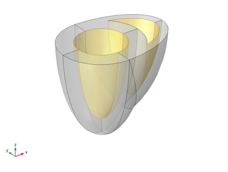
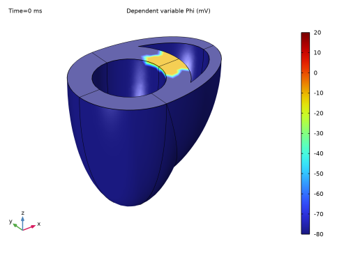
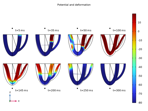
An initial pulse of electric potential (−10 mV) is applied on a rectangular area on the basal surface between the ventricles (Figure 6).

Figure 6: Initial impulse at the atrioventricular node.

Results and Discussion

The model computes the contraction of the myocardium due to an electric stimulus. Figure 5 displays the fibers layout in the undeformed configuration.

Figure 7 shows the time variation of the electric potential distribution and the deformation of the cardiac walls. The depolarization of the cells produces an active stress that causes the myocardium to contract. There is an upward motion of the apex and a small torsion of the ventricles. The heart returns to its original state after 300 ms.

Figure 7: Depolarization and repolarization of the cardiac walls at different times during the cardiac cycle.

Figure 8 shows the activation potential at three different points. Note that the last cells to depolarize are the first ones to repolarize. This effect is achieved by manipulating the dimensionless time constant as shown in Equation 4.

Figure 9 shows the internal volume variation of the left and right ventricles. Both chambers contract during the depolarization of the excited myocardial cells, thus reducing the internal volume. Then, the ventricles gradually return to their initial configuration to be again excited during the next heartbeat.

Figure 8: Plot of the activation duration at different locations.

Figure 9: Volume variation of the left and right ventricular chambers.

References

1. A.A. Bakir, A.A. Abed, M.C. Stevens, N.H. Lovell, and S. Dokos, “A Multiphysics Biventricular Cardiac Model: Simulations With a Left-Ventricular Assist Device,” Front. Physiol., vol. 9, p. 1259, 2018.

2. S. Göktepe and E. Kuhl, “Electromechanics of the heart: a unified approach to the strongly coupled excitation-contraction problem,” Comput. Mech., vol. 45, pp. 227–243, 2010.

3. M.P. Nash and A.V. Panfilov, “Electromechanical model of excitable tissue to study reentrant cardiac arrhythmias,” Prog. Biophys. Mol. Biol., vol. 85,pp. 501–522, 2004.

Notes About the COMSOL Implementation

The analysis is performed in two separated studies. In the first study the fiber orientation is computed. In a second study, the cardiac contraction following an electrical excitation is analyzed. In particular, the following steps are taken:

•

The fibers paths are computed using the and interfaces.

•

The contribution of the electrophysiology model (PDE interfaces) is included in the Solid Mechanics interface through the feature.

•

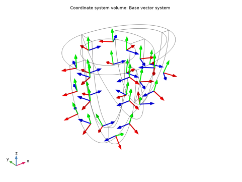
The feature is set up using the curvilinear fiber orientation.

•

The fiber pattern is displayed for postprocessing.

The distances Depi and Dendo used in Equation 1 to compute the dimensionless parameter β are determined by two interfaces. In one case the wall represents the endocardium, and in the other it represents the epicardium.

Inertial terms are neglected as reported in Ref. 2. The is set to in the interface setting.

The active stress (Equation 6) is added to the total stress with the feature. The fiber coordinate system is selected in the section.

In the settings for the feature, select the appropriate as a reference coordinate system. Then, in the section, select the orientation of the fiber (a0) to be aligned with the .

The feature automatically computes the corresponding invariants, for instance Ia as used in Equation 8, in order to compute the strain energy function Wani as in Equation 7.

The option is activated by default for the HGO model, and it evaluates the fibers’ strain energy to zero if the fiber stretch is in compression. This means that the fibers contribute to tensile stresses only.

The model parameters taken from literature references already include the effect of the membrane surface to volume ratio, χm, and the membrane capacitance, Cm. For this reason, these two parameters are set equal to 1 in this example.

The internal volume of the two ventricles is computed through the feature.

Nonlinear_Structural_Materials_Module/Hyperelasticity/biventricular_cardiac_model

Modeling Instructions

From the menu, choose .

New

In the window, click

Model Wizard

In the window, click

In the tree, select > .

Click .

In the tree, select > .

Click .

Click

In the tree, select > .

Click

Geometry 1

Set Geometry representation to to build the geometry correctly.

In the toolbar, click and choose .

Browse to the model’s Application Libraries folder and double-click the file biventricular_cardiac_model_geom_sequence.mph.

In the toolbar, click

Click the

button in the toolbar.

Complete geometry instructions can be found in the Appendix — Geometry Modeling Instructions section.

Global Definitions

Heart Geometry Parameters

In the window, under click .

In the window for , type Heart Geometry Parameters in the text field.

Definitions

Create selections to identify the basal surface, the epicardium and the endocardium.

Basal Surface

In the toolbar, click

In the window for , type Basal Surface in the text field.

Locate the section. From the list, choose .

Click the

button in the toolbar.

Select Boundaries 1, 3, 9, and 17 only.

LV-Endocardium

In the toolbar, click

In the window for , type LV-Endocardium in the text field.

Locate the section. From the list, choose .

Select Boundaries 6, 7, 12, and 16 only.

RV-Endocardium

In the toolbar, click

In the window for , type RV-Endocardium in the text field.

Locate the section. From the list, choose .

Select Boundaries 20 and 22 only.

Epicardium

In the toolbar, click

In the window for , type Epicardium in the text field.

Locate the section. From the list, choose .

Select Boundaries 4, 5, 10, 11, 15, 18, 19, and 21 only.

Endocardium

In the toolbar, click

In the window for , type Endocardium in the text field.

Locate the section. From the list, choose .

Locate the section. Under , click

In the dialog, in the list, choose and .

Click .

Global Definitions

Structural Mechanics Parameters

In the toolbar, click

and choose > .

In the window for , type Structural Mechanics Parameters in the text field.

Locate the section. Click

Browse to the model’s Application Libraries folder and double-click the file biventricular_cardiac_model_mechanical_passive_parameters.txt.

Electrical Parameters

In the toolbar, click

and choose > .

In the window for , type Electrical Parameters in the text field.

Locate the section. Click

Browse to the model’s Application Libraries folder and double-click the file biventricular_cardiac_model_electrical_parameters.txt.

Active Stress Parameters

In the toolbar, click

and choose > .

In the window for , type Active Stress Parameters in the text field.

Locate the section. Click

Browse to the model’s Application Libraries folder and double-click the file biventricular_cardiac_model_active_stress_parameters.txt.

Conversion Factors Parameters

In the toolbar, click

and choose > .

In the window for , type Conversion Factors Parameters in the text field.

Locate the section. Click

Browse to the model’s Application Libraries folder and double-click the file biventricular_cardiac_model_conversion_parameters.txt.

To compute the orientation of the fibers in any point in the myocardium it is necessary to know its distance from both the epicardium and the endocardium.

Wall Distance: Epicardium

In the window, under click .

In the window for , type Wall Distance: Epicardium in the text field.

Wall 1

In the toolbar, click

and choose .

In the window for , locate the section.

From the list, choose .

Wall Distance: Endocardium

In the window, under click .

In the window for , type Wall Distance: Endocardium in the text field.

In the toolbar, click

and choose .

In the window for , locate the section.

From the list, choose .

Assuming that the sheets are oriented perpendicularly to the wall, their direction can be found by computing the transmural direction.

Sheet Direction

In the window, under click .

In the window for , type Sheet Direction in the text field.

Locate the section. Select the checkbox.

Coordinate System Settings 1

In the window, under > click .

In the window for , locate the section.

From the list, choose .

Diffusion Method 1

In the toolbar, click

and choose .

Inlet 1

In the toolbar, click

and choose .

In the window for , locate the section.

From the list, choose .

Diffusion Method 1

In the window, click .

Outlet 1

In the toolbar, click

and choose .

In the window for , locate the section.

From the list, choose .

Mesh 1

In the window, under click .

In the window for , locate the section.

From the list, choose .

Click

The first study is used to obtain the sheets’ direction and the distance from the walls. These quantities can be used to find the fibers’ direction.

Study: Fiber Direction

In the window, click .

In the window for , type Study: Fiber Direction in the text field.

In the toolbar, click

Results

Wall Distance: Epicardium

In the window for , type Wall Distance: Epicardium in the text field.

Wall Distance: Endocardium

In the window, under click .

In the window for , type Wall Distance: Endocardium in the text field.

Coordinate system (cc), Vector Field (cc), Wall Distance: Endocardium, Wall Distance: Epicardium

In the window, under , Ctrl-click to select , , , and .

Right-click and choose .

Study: Fiber Direction

In the window for , type Study: Fiber Direction in the text field.

Add variables related to the fibers orientation.

Definitions

Fiber Orientation

In the window, under right-click and choose .

In the window for , type Fiber Orientation in the text field.

Locate the section. Click

Browse to the model’s Application Libraries folder and double-click the file biventricular_cardiac_model_fibers.txt.

The fibers reference system is obtained by rotating the curvilinear coordinate system found in the previous study.

Rotated System 2 (sys2)

In the toolbar, click

and choose .

In the window for , locate the section.

Find the subsection. In the β text field, type theta.

Fiber Reference System

In the toolbar, click

and choose .

In the window for , type Fiber Reference System in the text field.

Locate the section. From the list, choose .

From the list, choose .

Create a cylindrical system for postprocessing purposes.

Cylindrical System 4 (sys4)

In the toolbar, click

and choose .

In the window for , locate the section.

From the list, choose .

Boundary System 1 (sys1), Curvilinear System (cc) (cc_cs), Cylindrical System 4 (sys4), Fiber Reference System (sys3), Rotated System 2 (sys2)

In the window, under > , Ctrl-click to select , , , , and .

Right-click and choose .

Coordinate Systems

In the window for , type Coordinate Systems in the text field.

In the window, collapse the node.

Now we have all information needed to simulate the contraction. Add a Solid Mechanics interface and three PDE interfaces. The three PDEs will be used to solve the monodomain equation and to compute the active stress.

Add Physics

In the toolbar, click

to open the window.

Go to the window.

In the tree, select > .

Find the subsection. In the table, clear the checkbox for .

Click the button in the window toolbar.

In the tree, select > > .

In the table, clear the checkbox for .

Click the button in the window toolbar.

In the tree, select > > .

In the table, clear the checkbox for .

Click the button in the window toolbar.

In the tree, select > > .

In the table, clear the checkbox for .

Click the button in the window toolbar.

In the toolbar, click

to close the window.

Solid Mechanics (solid)

In the window for , locate the section.

From the list, choose .

Click to expand the section. From the list, choose .

Hyperelastic Material 1

In the toolbar, click

and choose .

In the window for , locate the section.

From the list, choose .

Fiber 1

In the toolbar, click

and choose .

Materials

Material 1 (mat1)

In the window, under right-click and choose .

In the window for , locate the section.

In the table, enter the following settings:


Property	Variable	Value	Unit	Property group
Lamé parameter λ	lambLame	lambda_lame	N/m²	Lamé parameters
Lamé parameter μ	muLame	mu_lame	N/m²	Lamé parameters
Density	rho	rhos	kg/m³	Basic
Fiber stiffness	k1HGO	af	Pa	Holzapfel-Gasser-Ogden
Model parameter	k2HGO	bf	1	Holzapfel-Gasser-Ogden
Fiber dispersion	k3HGO	0	1	Holzapfel-Gasser-Ogden

Electrophysiology: Transmembrane Potential (Phi)

In the window, under click .

In the window for , type Electrophysiology: Transmembrane Potential (Phi) in the text field.

Locate the section. Click

In the dialog, type electricpotential in the text field.

In the tree, select > .

Click .

In the window for , locate the section.

In the table, enter the following settings:


Source term quantity	Unit
Custom unit	A/m^3

Click to expand the section. From the list, choose .

From the list, choose .

Click to expand the section. In the text field, type Phi.

In the table, enter the following settings:


Phi

Electrophysiology: Conductance of Slow Processes (r)

In the window, under click .

In the window for , type Electrophysiology: Conductance of Slow Processes (r) in the text field.

Locate the section. In the table, enter the following settings:


Source term quantity	Unit
Custom unit	1/s

Locate the section. From the list, choose .

From the list, choose .

Locate the section. In the text field, type r.

In the table, enter the following settings:


r

Active Stress (Sa)

In the window, under click .

In the window for , type Active Stress (Sa) in the text field.

Locate the section. Click

In the dialog, type stress in the text field.

In the tree, select > .

Click .

In the window for , locate the section.

In the table, enter the following settings:


Source term quantity	Unit
Custom unit	N/m^2/s

Locate the section. From the list, choose .

From the list, choose .

Locate the section. In the text field, type Sa.

In the table, enter the following settings:


Sa

Definitions

Electrophysiology Variables

In the window, under right-click and choose .

In the window for , type Electrophysiology Variables in the text field.

Locate the section. Click

Browse to the model’s Application Libraries folder and double-click the file biventricular_cardiac_model_electrophysiology.txt.

Define the partial differential equations to solve in order to obtain the active stress.

Electrophysiology: Transmembrane Potential (Phi) (c)

Coefficient Form PDE 1

In the window, under > click .

In the window for , locate the section.

From the list, choose .

Specify the c matrix as


D_iso+DfibXX	DfibXY	DfibXZ
DfibXY	D_iso+DfibYY	DfibYZ
DfibXZ	DfibYZ	D_iso+DfibZZ

Locate the section. In the f text field, type -Chi_m*(Ie+Im).

Locate the section. In the da text field, type Chi_m*Cm.

Initial Values 1

In the window, click .

In the window for , locate the section.

In the Phi text field, type Phir+70[mV]*(Z>-1e-4[mm])*(X<31[mm])*(X>0[mm])*(Y>-10[mm])*(Y<10[mm]).

Electrophysiology: Conductance of Slow Processes (r) (c2)

Coefficient Form PDE 1

In the window, under > click .

In the window for , locate the section.

In the c text field, type 0.

Locate the section. In the a text field, type (1/betat)*(gamma+(mu1/(phi+mu2))*c*phi*(phi-b-1)).

Locate the section. In the f text field, type (1/betat)*(-gamma*c*phi*(phi-b-1)-mu1/(phi+mu2)*r^2).

Active Stress (Sa) (c3)

In the window, under > click .

In the window for , locate the section.

In the c text field, type 0.

Locate the section. In the a text field, type eps_delay.

Locate the section. In the f text field, type eps_delay*kT*(Phi-Phir).

Solid Mechanics (solid)

Fiber 1

In the window, under > > click .

In the window for , locate the section.

From the list, choose .

Locate the section. From the a list, choose .

The coupling between the potential and the deformation is obtained through the active stress. The active stress is added as an external stress. Use the fiber coordinate system to easily input the components.

Hyperelastic Material 1

In the window, click .

External Stress 1

In the toolbar, click

and choose .

In the window for , locate the section.

From the list, choose .

Locate the section. From the list, choose .

Specify the Sext matrix as


vs*Sa	0	0
0	vn*Sa	0
0	0	vf*Sa

Prescribed Displacement 1

In the toolbar, click

and choose .

In the window for , locate the section.

From the list, choose .

Locate the section. From the list, choose .

From the list, choose .

Add two nodes to compute the internal volumes of the left and right chambers during contraction using Gauss’s law. Since no internal fluid pressure is modeled, remove the subnode.

Enclosed Cavity 1

In the toolbar, click