PDF

Vacuum Drying
Introduction
Vacuum drying is a chemical process frequently used in the pharmaceutical and food industries to remove water or an organic solvent from a wet powder. When designing a vacuum drying system, engineers aim to minimize the drying time while maintaining high quality in the product. This model investigates vacuum drying in a Nutsche filter-dryer, which consists of a cylindrical drum filled with wet cake as seen in Figure 1. The top of the cake is exposed to a low pressure head space, and the side and bottom walls are exposed to heating fluid. By operating at a very low pressure and an elevated temperature, the evaporation rate of the liquid increases, thus accelerating the drying process of the powder. By modeling the heat transfer and evaporation of the solvent in the powder, the temperature and liquid phase profiles can be studied.
This example is based on the paper published by Murru and others for a powder dried with n-propanol under static conditions (Ref. 1).
Figure 1: Vacuum drying in an axisymmetric Nutsche filter dryer (Ref. 1).
Model Definition
The cylindrical cake can be modeled using a rectangular geometry in a 2D axisymmetric component. The cake radius is 40 cm and the cake height is 10 cm.
The vacuum drying process involves heat transfer and vapor transport in modeling the evaporation of the solvent. This example simulates the heat transfer through the cake using the Heat Transfer in Solids interface and the volume fraction of solvent using a Coefficient Form PDE interface. A predefined moisture transport in porous media physics interface is available in the Heat Transfer Module.
Heat flux boundary conditions are defined on the side and bottom boundaries to account for the external heating fluid. The evaporation of solvent is captured in two ways: a heat sink term to account for the energy lost from the cake as the liquid solvent changes to vapor phase, and a mass sink term to account for the loss of solvent in the cake.
Liquid phase evaporation
The equation in the Coefficient Form PDE interface solves for the volume fraction of liquid, θL, in the cake:
where DL is the apparent liquid diffusion coefficient, is the evaporation rate, and ρL is the liquid phase density.
The source term accounts for the loss of solvent as it evaporates. All boundaries are prescribed as no flux conditions.
The evaporation rate is related to the difference in the equilibrium vapor pressure of the gas in the cake and head space vapor pressure pG with:
, if
, if or
where is the evaporation rate constant (1/s). In this case, the head space pressure, or the vacuum pressure surrounding the cake, is set to be 15 mbar.
Evaporation should cease once the value of liquid phase reaches zero (fully evaporated) or if the local vapor pressure does not exceed the head space vapor pressure (no driving force for the evaporation). In the model, step functions are used to smoothly ramp the evaporation rate down to zero under these conditions.
The equilibrium vapor pressure of n-propanol, which is related to the temperature (T), can be found using Antoine’s equation: where A, B, and C are constants found in Ref. 2.
The solvent migrates in the cake due to capillary flow. Instead of directly solving for the velocity field of the liquid phase in the porous media, the transport of the solvent through the cake can be approximated as a diffusion process. Therefore, when there is a gradient in the volume fraction of solvent, the liquid phase migrates from the region with a high volume fraction of solvent to the region with a low volume fraction of solvent. The liquid diffusion coefficient is calculated with:
, if
, if
where is the residual saturation and is the proportionality constant, both of which are determined experimentally in Ref. 1. When the volume fraction of liquid phase present is below the critical value of , then diffusion of the solvent in the cake should no longer occur. In the model, a step function is used to smoothly ramp the diffusion coefficient down to zero under these conditions.
As the cake dries, the liquid phase evaporates and is replaced by gas between the solid particulates. The sum of the volume fractions of the three phases should equal unity. Therefore, the volume fraction of gas present (θG) can be calculated with respect to the constant volume fraction of solid powder (θS) and the variable liquid volume fraction (θL) with .
Heat transfer
The equations in the Heat Transfer in Solids interface solve for the temperature, T, in the cake:
where ρeff is the density (SI unit: kg/m^3), Cp is the heat capacity (SI unit: J/(kg*K)), λeff is the thermal conductivity (SI unit: W/(m*K)), and Q is the heat source (SI unit: W/m3).
Energy is required for evaporation to occur, which is characterized in a heat source domain condition with , where is the latent heat of vaporization (SI unit: J/kg) found in Ref. 3.
The side and bottom boundaries of the filter-dryer are exposed to a heating fluid. In this model, heat flux boundary conditions account for the energy transferred to the cake from heating fluid given a heat transfer coefficient of 10 W/(m^2*K).
The cake consists of solid powder particulates, a liquid solvent, and a gas that fills the voids between the solid powder particulates. Therefore, the material properties of the cake must take into account the properties of the 3 phases in proportion to their presence in the cake. In this case, the effective density and effective heat capacity are calculated with:
where θL, θS, and θG represent the volume fraction of the liquid, solid, and gas phases in the cake, respectively. The material properties of the liquid phase (ρL and ) are taken from Ref. 4 for n-propanol at a temperature of . Solid powder properties are found in Ref. 1.
The effective thermal conductivity is calculated with:
where and are the thermal conductivities of the dry and fully saturated cake, respectively, found in Ref. 1. Instead of writing user defined expressions for the effective material properties of the cake, the Multiphase Material is used.
Results and Discussion
The following figures show the temperature (Figure 2), volume fraction of liquid phase (Figure 3), and the apparent moisture diffusivity (Figure 4) in the cake after 30 hours. The temperature of the cake approaches the temperature of the heating fluid ( or 333.15 K) at the bottom and side boundaries, as seen in Figure 2. Because the liquid phase evaporates in the heated region, the volume fraction of the liquid phase is lowest near the heated side and bottom boundaries and highest in the center of the cake, as seen in Figure 3. The apparent moisture diffusivity is also highest in the center of the cake where liquid phase has not yet evaporated and approaches zero in areas where the liquid phase has already evaporated, as seen in Figure 4.
The evaporation rate after 10, 20, and 30 hours is shown in Figure 5, Figure 6, and Figure 7. The evaporation front starts near the side and bottom walls where the cake is heated. As the amount of solvent present near these boundaries decreases, the evaporation rate decreases in turn, shifting the evaporation front toward the center of the cake.
Figure 2: Temperature in the cake after 30 hours.
Figure 3: Volume fraction of liquid phase in the cake after 30 hours.
Figure 4: Apparent moisture diffusivity in the cake after 30 hours.
Figure 5: Evaporation rate after 10 hours.
Figure 6: Evaporation rate after 20 hours.
Figure 7: Evaporation rate after 30 hours.
References
1. M. Murru and others, “Model-based scale-up of vacuum contact drying of pharmaceutical compounds,” Chem. Eng. Sci., vol. 66, pp. 5045–5054, 2011.
2. H.R. Kemme and S.I. Kreps, “Vapor Pressure of Primary n-Alkyl Chlorides and Alcohols,” J. Chem. Eng. Data, vol. 14, no. 1, pp. 98–102. 1969.
3. I.M. Smallwood, Handbook of Organic Solvent Properties, Arnold, 1996.
4. “n-Propanol”, BASF, Technical Leaflet, March 2008.
Application Library path: COMSOL_Multiphysics/Chemical_Engineering/vacuum_drying
Modeling Instructions
From the File menu, choose New.
New
In the New window, click  Model Wizard.
Model Wizard
1
In the Model Wizard window, click  2D Axisymmetric.
2
In the Select Physics tree, select Heat Transfer > Heat Transfer in Solids (ht).
3
Click Add.
Also add a PDE interface to solve for the volume fraction of liquid in the cake.
4
In the Select Physics tree, select Mathematics > PDE Interfaces > Coefficient Form PDE (c).
5
Click Add.
6
In the Field name (1) text field, type theta.
7
In the Dependent variables (1) table, enter the following settings:
8
In the Source term quantity table, enter the following settings:
9
Click  Study.
10
In the Select Study tree, select General Studies > Time Dependent.
11
The list of parameters and variables are imported from files available in the Application Libraries folder.
Global Definitions
Parameters 1
1
In the Model Builder window, under Global Definitions click Parameters 1.
2
In the Settings window for Parameters, locate the Parameters section.
3
Click  Load from File.
4
Definitions
Variables 1
1
In the Model Builder window, under Component 1 (comp1) right-click Definitions and choose Variables.
2
In the Settings window for Variables, locate the Variables section.
3
Click  Load from File.
4
Next, define two step functions to smoothly decrease the evaporation rate and apparent moisture diffusivity to zero as the solvent evaporates.
Step 1 (step1)
1
In the Definitions toolbar, click  More Functions and choose Step.
2
In the Settings window for Step, locate the Parameters section.
3
In the Location text field, type 1.005.
4
Click to expand the Smoothing section. In the Size of transition zone text field, type 0.01.
Step 2 (step2)
1
In the Definitions toolbar, click  More Functions and choose Step.
2
In the Settings window for Step, locate the Parameters section.
3
In the Location text field, type 0.005.
4
Locate the Smoothing section. In the Size of transition zone text field, type 0.01.
Geometry 1
Rectangle 1 (r1)
1
In the Geometry toolbar, click  Rectangle.
2
In the Settings window for Rectangle, locate the Size and Shape section.
3
In the Width text field, type R0.
4
In the Height text field, type H0.
5
Click  Build All Objects.
6
Click the  Zoom Extents button in the Graphics toolbar.
Materials
Multiphase Material 1 (mpmat1)
In the Model Builder window, under Component 1 (comp1) right-click Materials and choose More Materials > Multiphase Material.
Constrained Gas Phase
1
In the Model Builder window, under Component 1 (comp1) > Materials > Multiphase Material 1 (mpmat1) click Phase 1 (mpmat1.phase1).
2
In the Settings window for Phase, type Constrained Gas Phase in the Label text field.
3
Locate the Material Contents section. In the table, enter the following settings:
Liquid Phase
1
In the Model Builder window, right-click Multiphase Material 1 (mpmat1) and choose Phase.
2
In the Settings window for Phase, type Liquid Phase in the Label text field.
3
Locate the Volume Fraction section. In the Vf text field, type thetaL.
4
Locate the Material Contents section. In the table, enter the following settings:
Solid Phase
1
Right-click Multiphase Material 1 (mpmat1) and choose Phase.
2
In the Settings window for Phase, type Solid Phase in the Label text field.
3
Locate the Volume Fraction section. In the Vf text field, type thetaS.
4
Locate the Material Contents section. In the table, enter the following settings:
Heat Transfer in Solids (ht)
Heat Source 1
1
In the Physics toolbar, click  Domains and choose Heat Source.
2
3
In the Settings window for Heat Source, locate the Heat Source section.
4
In the Q0 text field, type -mdot*deltaH.
Heat Flux 1
1
In the Physics toolbar, click  Boundaries and choose Heat Flux.
2
3
In the Settings window for Heat Flux, locate the Heat Flux section.
4
From the Flux type list, choose Convective heat flux.
5
In the h text field, type hq.
6
In the Text text field, type Th.
Initial Values 1
1
In the Model Builder window, click Initial Values 1.
2
In the Settings window for Initial Values, locate the Initial Values section.
3
In the T text field, type T0.
Next, define the Coefficient Form PDE interface for the liquid phase evaporation.
Coefficient Form PDE (c)
Coefficient Form PDE 1
1
In the Model Builder window, under Component 1 (comp1) > Coefficient Form PDE (c) click Coefficient Form PDE 1.
2
In the Settings window for Coefficient Form PDE, locate the Diffusion Coefficient section.
3
In the c text field, type DL.
4
Locate the Source Term section. In the f text field, type -mdot/rhoL.
Initial Values 1
1
In the Model Builder window, click Initial Values 1.
2
In the Settings window for Initial Values, locate the Initial Values section.
3
In the thetaL text field, type thetaL0.
Set the mesh to Extremely fine to better resolve the evaporation front in the domain.
Mesh 1
1
In the Model Builder window, under Component 1 (comp1) click Mesh 1.
2
In the Settings window for Mesh, locate the Physics-Controlled Mesh section.
3
From the Element size list, choose Extremely fine.
4
Click  Build All.
Study 1
Solution 1 (sol1)
1
In the Study toolbar, click  Show Default Solver.
The dependent variable scaling for thetaL is manually set to 0.5. This provides a better convergence.
2
In the Model Builder window, expand the Solution 1 (sol1) node.
3
In the Model Builder window, expand the Study 1 > Solver Configurations > Solution 1 (sol1) > Dependent Variables 1 node, then click Dependent Variable ThetaL (comp1.thetaL).
4
In the Settings window for Field, locate the Scaling section.
5
From the Method list, choose Manual.
6
In the Scale text field, type 0.5.
Step 1: Time Dependent
1
In the Model Builder window, under Study 1 click Step 1: Time Dependent.
2
In the Settings window for Time Dependent, locate the Study Settings section.
3
From the Time unit list, choose h.
4
In the Output times text field, type range(0,1,70).
5
In the Study toolbar, click  Compute.
Results
Temperature (ht)
1
In the Settings window for 2D Plot Group, locate the Color Legend section.
2
Select the Show units checkbox.
3
Locate the Data section. From the Time (h) list, choose 30.
4
In the Temperature (ht) toolbar, click  Plot.
Coefficient Form PDE 1
1
In the Model Builder window, click Coefficient Form PDE 1.
2
In the Settings window for 3D Plot Group, locate the Data section.
3
From the Time (h) list, choose 30.
4
In the Coefficient Form PDE 1 toolbar, click  Plot.
Result Templates
1
In the Results toolbar, click  Result Templates to open the Result Templates window.
2
Go to the Result Templates window.
3
In the tree, select Study 1/Solution 1 (sol1) > Heat Transfer in Solids > Temperature (ht).
4
Click the Add Result Template button in the window toolbar.
5
In the Results toolbar, click  Result Templates to close the Result Templates window.
Results
Temperature (ht) 1
1
In the Settings window for 3D Plot Group, locate the Color Legend section.
2
Select the Show units checkbox.
Apparent moisture diffusivity
1
In the Results toolbar, click  2D Plot Group.
2
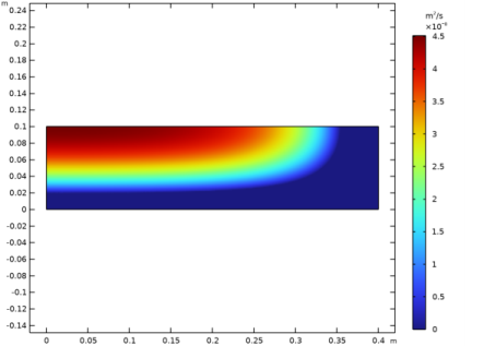
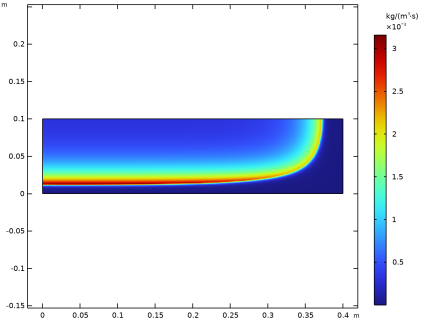
In the Settings window for 2D Plot Group, type Apparent moisture diffusivity in the Label text field.
3
Locate the Data section. From the Time (h) list, choose 30.
4
Locate the Color Legend section. Select the Show units checkbox.
Surface 1
1
Right-click Apparent moisture diffusivity and choose Surface.
2
In the Settings window for Surface, locate the Expression section.
3
In the Expression text field, type DL.
4
In the Apparent moisture diffusivity toolbar, click  Plot.
Evaporation rate
1
In the Results toolbar, click  2D Plot Group.
2
In the Settings window for 2D Plot Group, type Evaporation rate in the Label text field.
3
Locate the Data section. From the Time (h) list, choose 30.
4
Locate the Color Legend section. Select the Show units checkbox.
Surface 1
1
Right-click Evaporation rate and choose Surface.
2
In the Settings window for Surface, locate the Expression section.
3
In the Expression text field, type mdot.
4
In the Evaporation rate toolbar, click  Plot.