PDF

A Tubular Reactor Surrogate Model
Introduction
This example demonstrates how to increase the computational speed of a tubular reactor app by using a surrogate model, as opposed to a finite element model. A surrogate model is a simpler, usually computationally cheaper model, which is used to approximate the behavior of a more complex, and often more computationally expensive, model. The faster model evaluation offered by the surrogate model provides the user of the app a more interactive user experience and makes it easier to spread the use of simulations in an organization.
This document shows how to create the surrogate model by training a deep neural network (DNN). The design of the app that uses this surrogate model is described in a separate document.
The surrogate model training is based on output data from a large parametric sweep of the embedded tubular reactor model. In order to make this parametric sweep efficient, a design of experiments method is used.
The surrogate model presented here extends on the model Tubular Reactor with Nonisothermal Cooling Jacket available in the Application Libraries at
COMSOL_Multiphysics/Chemical_Engineering/tubular_reactor
The corresponding app extends on the tubular reactor app available in the Application Libraries at
COMSOL_Multiphysics/Applications/tubular_reactor
The extended app that uses the surrogate model is available at
COMSOL_Multiphysics/Applications/tubular_reactor_surrogate
Model Definition
The app is based on a model of a tubular reactor, which is used to analyze an elementary, exothermic, and irreversible reaction. The reactions take place in a liquid phase and the reactor is operating in the laminar flow regime. Temperature control is maintained via a cooling jacket and the model focuses on the steady-state behavior of the reactor.
The reaction is a conversion of chemical species A, B, and C in a liquid:
(1)
Here, A represents propylene oxide, B represents water, and C represents propylene glycol. The reaction kinetics are first order in regard to the concentration of species A.
Figure 1 describes the reactor model.
Figure 1: Schematic of the reactor model.
Inputs and Outputs
The simulation is used to analyze the compositional variations in both the radial and axial directions. The results include the spatial distribution of the temperature and the chemical species concentrations, as well as various quantities that can be derived from these. In the app, the results are limited to the temperature and the conversion factor of species A. The conversion factor ranges from 0 to 1, indicating the extent of the conversion of species A into species C. A factor of 0 signifies no conversion, while a factor of 1 represents complete conversion into Species C.
The app has three scalar inputs:
In order to train the surrogate model, two additional inputs are needed: the radial, r, and axial, z, coordinates in a cylindrical coordinate system.
The two outputs, temperature, T, and conversion factor, xA, are then viewed as functions of the five inputs:
T = f(rzEkdHrx)
xA = g(rzEkdHrx)
In a traditional model, the finite element solution would provide us with the functions f and g. However, here we replace the finite element model with a surrogate model consisting of two new functions fs and gs (using the subscript “s” for surrogate), which will approximate the finite element solution and be much faster to evaluate:
T = fs(rzEkdHrx)
xA = gs(rzEkdHrx)
Note: In the user interface of the software, the surrogate model functions fs and gs are called dnn1_1 and dnn1_2 (see below).
Design of Experiments
In order to train the surrogate model, consisting of the functions fs and gs, a large number of data points are needed to fully reveal how the inputs (rzEkdHrx) map to the outputs T and xA. The full finite element model of the tubular reactor will need to be solved for each such data point in the five-dimensional input space defined by the input parameters. Although a straightforward parametric sweep could densely and uniformly distribute input points throughout a five-dimensional grid, such an approach would be inefficient. While random sampling may serve as an alternative, it has inherent drawbacks, such as nonuniform sampling and potential failure to cover the entire input space.
Instead, a more strategic approach is to use a design of experiments method, carefully sampling within the parameter space. In COMSOL Multiphysics, a dedicated Surrogate Model Training study uses Latin hypercube sampling (LHS), which is a design of experiments method that generates a dataset that uniformly covers the input space without requiring an excessive number of finite element computations. This is a clear advantage over uniform grid or random sampling. LHS is a more efficient method for data generation intended for the purpose of training a surrogate model.
The more data points that you use, the more accurately the surrogate model will be able to represent the actual solution. However, generating a large number of data points require a large number of simulations to be run, and there is a tradeoff between the time it takes to generate all the data points and the desired accuracy of the surrogate model.
In this example, the input parameters include the radial, r, and axial, z, coordinates and a Geometry Sampling feature is used in order to efficiently sample the coordinate space. For each set of scalar inputs, Ekand dHrx, generated by LHS, a table is generated with the values of the outputs T and xA, for all mesh points. All the computed data is stored in a table which is saved to file. This file can be embedded in the MPH-file or saved to the file system. The figure below shows a spreadsheet with the first portion of a table generated by the Surrogate Model Training study.
The first two columns contain the coordinate data, the next three columns contain the reaction-related input parameters, and the last two columns contain the output parameters.
The figure below shows the Geometry Sampling settings, available under Component 1>Definitions>Surrogate Model Sampling.
In this example, the solution is sampled in a 20-by-20 grid. For a more irregularly shaped geometry you can instead choose the option Geometric entity selection and thereby use the finite element mesh for sampling. There is also a third option, Mesh interpolation, if you rather want to use a separate mesh for the surrogate model interpolation.
The figure below shows the corresponding Surrogate Model Training study settings in the Model Builder.
In this example, the number of finite element solutions, or Number of input points, used for the data generation is set to 100. This number is chosen empirically to train the surrogate model to a sufficient degree of accuracy. The figure below shows the portion of the Surrogate Model Training study that includes the setting for the Number of input points.
Note, however, that the Number of input points only defines the number of LHS points. This number is then multiplied by the number of node points in the model, resulting in a data table stored as a CSV file in the model, containing approximately 40,000 rows. The CSV file is stored in the Application Builder workspace, under Libraries>Files.
If you have access to a cluster, then you can utilize parallelization to speed up the surrogate model data generation. This option is called Distribute model evaluation and is available in the Advanced Settings section of the Surrogate Model Training study window, as shown below.
To enable this option, select the Batch and Cluster option in the Show More Options dialog, as shown below.
Note also that for more robust training, select the option Skip problematic parameters for Error handling. This ensures that the training continues even if the model cannot be computed for certain sets of input parameters. For example, if a set of input parameters generates an invalid geometry model or mesh, or if the solver does not converge.
For more information on cluster settings, see the COMSOL Multiphysics Reference Manual.
Surrogate Models
The Surrogate Model Training study is used to generate the data needed for the training and includes the option of also setting up the surrogate model automatically after the data generation step. In this example, the latter option is not used but the study is only used for generating the data and, in a separate step, the surrogate model is created and trained based on this data. The surrogate model is available as a function in the Model Builder under Global Definitions. The figure below shows the Functions menu with the Deep Neural Network surrogate model highlighted.
Included with COMSOL Multiphysics is the Deep Neural Network (DNN) surrogate model. With the Uncertainty Quantification Module you will additionally get the surrogate models Gaussian Process (GP) and Polynomial Chaos Expansion (PCE). The GP and PCE surrogate models include uncertainty estimates in regards to the quality of the data fit whereas the DNN model does not give any uncertainty estimates. The benefit with the DNN model is that it can handle larger datasets than the GP and PCE models, which are both limited to 2000 input points (data points).
To get an intuitive feeling for the surrogate models you can think of them as a nonlinear generalization of the linear interpolation functions available in COMSOL Multiphysics. However, the linear interpolation functions can only handle three-dimensional inputs; in the case of spatial interpolation this would be the spatial coordinates x, y, and z. The methods used for linear interpolation do not easily generalize to higher-dimensional unstructured input data and it is hard to find efficient methods for linear interpolation in such cases. The surrogate models, on the other hand, can handle an arbitrary number of inputs. In addition, the surrogate models are well suited for handling complex nonlinear relationships in the data.
The Deep Neural Network Surrogate Model
A DNN model consists of an input layer, a series of hidden layers, and an output layer. Each layer consists of a number of nodes, or neurons. Figure 2 shows a graph for a network with three hidden layers, 5 input nodes, and 2 output nodes.
Figure 2: A neural network with five layers.
The network shown in the figure above could in principle be used for the tubular reactor model; however, it is a bit too simple to represent the model with enough accuracy. Instead, in the tubular reactor example, there are four hidden layers with 50, 40, 30, and 20 nodes, respectively.
The figure below shows the settings window for the surrogate model used in the tubular reactor example.
The Data source option supports referencing a Results table or a File. The File option supports data on the COMSOL spreadsheet format. In this example, the surrogate model functions for the temperature and conversion are called dnn1_1 and dnn1_2, respectively.
Note: You can differentiate these functions with respect to any of their input arguments. For example, d(dnn1_1(x1,x2,x3,x4,x5),x2) is the partial derivative of dnn1_1 with respect to the second input argument. This implies, among other things, that you can use the surrogate model functions for gradient-based optimization.
Choosing the number of layers and nodes in a neural network is often an iterative process that involves a combination of knowledge about the specific problem and data, empirical testing, and a bit of trial and error. A network with too few hidden layers or nodes may not be complex enough to serve as an accurate surrogate model. A network with too many hidden layers or nodes may suffer from so-called overfitting, where the network performs well on the training data but fails to generalize to a dataset that it was not trained on. A model with a large number of hidden layers or nodes will also be slower to evaluate than a lighter model.
Figure 3 shows two additional configurations of neural networks that can serve as inspiration for your own modeling projects:
Figure 3: Examples of deep neural network configurations.
In COMSOL Multiphysics, you define the number of output features from each layer, instead of defining the number of nodes. This means that, for the tubular reactor example, you specify 50,40, 30, and 20 for the hidden layers. The number of input and output features are automatically determined from the list of arguments and function values in the Column Settings section in the Settings window of the Deep Neural Network surrogate model.
Training the Surrogate Model
Associated with each edge in the neural network graph is a weight. When the neural network is trained on the data generated by the Surrogate Model Training study, the weights, together with other network parameters, called biases, are optimized so as to minimize the error between the surrogate model and the finite element model. This error is known as the loss function, L. The loss function can be of different kinds and the default setting is a root-mean-squared error (RMSE) loss function.
Based on the previously defined functions f, g, fs, and gs, we can write the RMSE loss function schematically as
where N is the number of training data points and validation data points corresponding to the training loss and validation loss, respectively.
In the Deep Neural Network Settings window, in the Training and Validation section, you can find the optimization solver parameters, also known as hyperparameters shown in the figure below.
Some of the most important parameters are the Learning rate, Batch size, and Number of epochs. The Learning rate, which can be likened in some ways to numerical damping in a nonlinear Newton solver, determines the step size during the optimization process. A learning rate that is too small can lead to the model getting stuck in a local minimum, while a learning rate that is too large can result in overshooting the minimum and poor convergence. The Batch size denotes how the training data is divided up into subsets during the optimization process. A too small batch size can lead to noisy gradient updates and longer training times, while a too large batch size might lead to poor generalization and inefficient utilization of computational resources. The Number of epochs, which defines the number of complete passes through the entire dataset, plays an important role in the learning process. Too few epochs can result in underfitting, where the model has not adequately learned from the training data, while too many epochs can lead to overfitting, where the model learns the noise in the training data and performs poorly on new, unseen data. In this example, the Number of epochs is empirically set to 50000 and the other parameters are left at their default values.
To train the surrogate model you click the Train Model button at the top of the Deep Neural Network Settings window. During the training process, you can monitor the progress in terms of the loss function versus epoch in the Convergence Plot window, as shown in Figure 4 below after 3000 epochs.
Figure 4: Training and validation losses after 3000 epochs.
The convergence plot shows two versions of the loss function: the Training loss and the Validation loss. The Training loss shows the loss function with respect to the main part of the training data created by the Surrogate Model Training study. A random portion of the data is set aside and treated as unseen data for validation purposes and this is what the Validation loss represents.
In more detail, the training loss measures how well the neural network fits the training data. It decreases as the model learns during training. However, if it becomes too low, the model might be overfitting, meaning it is learning the training data too closely and may perform poorly on unseen data.
The validation loss measures the model’s performance on the validation data. It gives an estimate of how well the model will generalize to new, unseen data. If validation loss starts increasing while training loss is still decreasing, it usually indicates overfitting.
The hyperparameters are tuned to find a balance where both training and validation loss are minimized, indicating the model has learned well and can also generalize well to new data.
Note that if you have very few data points, you will not see the convergence graph but only the contents of the Information section in the Deep Neural Network settings window, as shown below.
Results and Discussion
The results plots are similar to the model Tubular Reactor with Nonisothermal Cooling Jacket. However, instead of 2D plots this model includes the temperature and conversion as revolved 3D plots. In addition, the corresponding revolved plots for the surrogate model are included (not shown here).
The revolved plots Figure 5 and Figure 6 show the computed temperature and conversion, respectively. These plots show that where the temperature is low, little conversion takes place and vice versa. This is because the rate of the reaction is temperature dependent. The low temperature closest to the wall is due to the coolant. The surrogate model plots are virtually identical in appearance (not shown here).
Figure 5: Computed temperature.
Figure 6: Computed conversion.
The computed temperature and conversion surface profiles at the outlet are shown below together with the profiles predicted by the surrogate model. The plots corresponding to the finite element solution is labeled “computed” and the plots corresponding to the surrogate model is labeled “preview”. The term preview comes from the fact that the surrogate model plots are used as preview plots in the corresponding app where this model is used as the embedded model.
Figure 7: Computed and predicted temperature profiles at the outlet.
Figure 8: Computed and predicted conversion profiles at the outlet.
Application Library path: COMSOL_Multiphysics/Chemical_Engineering/tubular_reactor_surrogate
Modeling Instructions
Start by loading the original tubular reactor model.
Application Libraries
1
From the File menu, choose Application Libraries.
2
In the Application Libraries window, select COMSOL Multiphysics > Chemical Engineering > tubular_reactor in the tree.
3
Component 1 (comp1)
In the Model Builder window, expand the Component 1 (comp1) node.
Definitions
Define a Surrogate Model Sampling feature for Component I (comp I). This will enable sampling of field variables relative to a mesh or grid. In this case the grid option is used
Geometry Sampling 1
1
In the Model Builder window, expand the Component 1 (comp1) > Definitions node.
2
Right-click Definitions and choose Surrogate Model Sampling > Geometry Sampling.
3
In the Settings window for Geometry Sampling, locate the Sample Method section.
4
From the Sample method list, choose Grid.
5
Find the R subsection. In the Maximum text field, type 0.1.
6
In the Resolution text field, type 20.
7
Find the Z subsection. In the Resolution text field, type 20.
Study 1
Surrogate Model Training
1
In the Model Builder window, expand the Study 1 node.
2
Right-click Study 1 and choose More Study Extensions > Surrogate Model Training.
The quantities of interest will be the temperature, T, and conversion, xA, respectively, with values from the Domain Point Probes.
3
In the Settings window for Surrogate Model Training, locate the Quantities of Interest section.
4
Click  Add twice.
5
6
From the Geometry sampling list, choose Geometry Sampling 1.
7
8
From the Geometry sampling list, choose Geometry Sampling 1.
Next, define the input parameters E, ke, and dHrx. These represent the activation energy, thermal conductivity, and heat of reaction, respectively. Additionally, specify the parameter bounds. These values are taken from the original tubular reactor app. The number of sampled data points is 100.
9
Locate the Input Parameters section. Click  Add three times.
10
11
12
In the Lower bound text field, type 71518.
13
In the Upper bound text field, type 79205.
14
15
In the Lower bound text field, type 0.0559.
16
In the Upper bound text field, type 5.6.
17
18
In the Lower bound text field, type -101600.
19
In the Upper bound text field, type -67733.
20
Find the Sampling settings subsection. In the Number of input points text field, type 100.
21
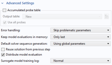
Locate the Advanced Settings section. From the Error handling list, choose Skip problematic parameters.
This setting makes the data generation stage more robust. Start generating the table with training data. Solving for 100 data points in a 20-by-20 grid will generate 40,000 data points and will take about 7 minutes on a moderately powerful workstation.
22
In the Study toolbar, click  Compute.
Define a Grid dataset for evaluating the surrogate model.
Results
Grid 2D 1
1
In the Model Builder window, expand the Results > Datasets node.
2
Right-click Results > Datasets and choose More 2D Datasets > Grid 2D.
3
In the Settings window for Grid 2D, locate the Data section.
4
From the Source list, choose Function.
5
Locate the Parameter Bounds section. Find the First parameter subsection. In the Name text field, type x1.
6
In the Maximum text field, type 0.1.
7
Find the Second parameter subsection. In the Name text field, type x2.
8
Click to expand the Grid section. In the x1 resolution text field, type 25.
9
In the x2 resolution text field, type 75.
Global Definitions
Deep Neural Network 1
1
In the Home toolbar, click  Functions and choose Global > Deep Neural Network.
2
In the Settings window for Deep Neural Network, locate the Layers section.
3
Click  Add Hidden Layer three times to add three hidden layers.
4
5
In the Output features text field, type 50.
6
7
In the Output features text field, type 40.
8
9
In the Output features text field, type 30.
10
11
In the Output features text field, type 20.
12
Locate the Data section. From the Data source list, choose Result table.
13
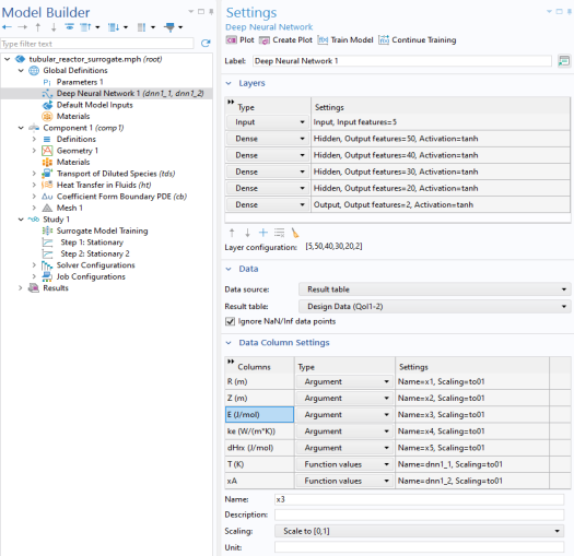
Locate the Data Column Settings section. In the table, enter the following settings:
14
15
In the Name text field, type dnn1_1.
16
17
In the Name text field, type dnn1_2.
18
Click  Train Model.
The training will take about 2 minutes on a moderately powerful workstation.
Study 1
Surrogate Model Training
1
In the Model Builder window, under Study 1 right-click Surrogate Model Training and choose Disable.
Disable the Surrogate Model Training study to prepare the model for being used as the embedded model in an app.
2
In the Study toolbar, click  Compute.
Results
Now, define a Mirror dataset, a Revolution dataset, and a Grid 1D dataset for the various visualizations. Then, define different plots for the temperature and conversion. The temperature and conversion fields are visualized in 3D using a Revolution dataset and in 1D along a radius at the outlet.
Mirror 2D 2
1
In the Results toolbar, click  More Datasets and choose Mirror 2D.
2
In the Settings window for Mirror 2D, locate the Data section.
3
From the Dataset list, choose Grid 2D 1.
Revolution 2D 3
1
In the Results toolbar, click  More Datasets and choose Revolution 2D.
2
In the Settings window for Revolution 2D, locate the Data section.
3
From the Dataset list, choose Grid 2D 1.
4
Click to expand the Revolution Layers section. In the Start angle text field, type -90.
5
In the Revolution angle text field, type 225.
Grid 2D 1
1
In the Model Builder window, click Grid 2D 1.
2
In the Settings window for Grid 2D, locate the Data section.
3
From the Function list, choose Deep Neural Network 1 (dnn1_1, dnn1_2).
4
In the Model Builder window, collapse the Results > Datasets node.
Temperature, 3D (Revolved)
1
In the Results toolbar, click  3D Plot Group.
2
In the Settings window for 3D Plot Group, type Temperature, 3D (Revolved) in the Label text field.
Surface 1
1
Right-click Temperature, 3D (Revolved) and choose Surface.
2
In the Settings window for Surface, locate the Expression section.
3
In the Expression text field, type T.
4
Locate the Coloring and Style section. From the Color table list, choose ThermalLight.
Temperature, 3D (Revolved)
1
In the Model Builder window, click Temperature, 3D (Revolved).
2
In the Temperature, 3D (Revolved) toolbar, click  Plot.
3
Click the  Zoom Extents button in the Graphics toolbar.
Compare this plot with that shown in Figure 5.
Temperature, 3D, Surrogate (Revolved)
1
In the Results toolbar, click  3D Plot Group.
2
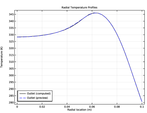
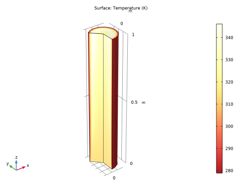
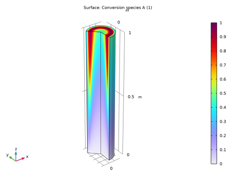
In the Settings window for 3D Plot Group, type Temperature, 3D, Surrogate (Revolved) in the Label text field.
3
Locate the Data section. From the Dataset list, choose Revolution 2D 3.
4
Locate the Plot Settings section. From the View list, choose View 3D 3.
Surface 1
1
Right-click Temperature, 3D, Surrogate (Revolved) and choose Surface.
The surrogate model for temperature is visualized by entering the expression for the corresponding function dnn1_1.
2
In the Settings window for Surface, locate the Expression section.
3
In the Expression text field, type dnn1_1(x1,x2,E,ke,dHrx).
4
Locate the Coloring and Style section. From the Color table list, choose ThermalLight.
Temperature, 3D, Surrogate (Revolved)
1
In the Model Builder window, click Temperature, 3D, Surrogate (Revolved).
2
In the Temperature, 3D, Surrogate (Revolved) toolbar, click  Plot.
Conversion, 3D (Revolved )
1
In the Results toolbar, click  3D Plot Group.
2
In the Settings window for 3D Plot Group, type Conversion, 3D (Revolved ) in the Label text field.
Surface 1
1
Right-click Conversion, 3D (Revolved ) and choose Surface.
2
In the Settings window for Surface, locate the Expression section.
3
In the Expression text field, type xA.
4
Click to expand the Range section. Select the Manual color range checkbox.
5
In the Maximum text field, type 1.
6
In the Conversion, 3D (Revolved ) toolbar, click  Plot.
The plot should resemble the one in Figure 6.
Conversion, 30, Surrogate
1
In the Results toolbar, click  3D Plot Group.
2
In the Settings window for 3D Plot Group, type Conversion, 30, Surrogate in the Label text field.
3
Locate the Data section. From the Dataset list, choose Revolution 2D 3.
4
Locate the Plot Settings section. From the View list, choose View 3D 3.
Surface 1
1
Right-click Conversion, 30, Surrogate and choose Surface.
The surrogate model for conversion is visualized by entering the expression for the corresponding function dnn1_2.
2
In the Settings window for Surface, locate the Expression section.
3
In the Expression text field, type dnn1_2(x1,x2,E,ke,dHrx).
4
Locate the Range section. Select the Manual color range checkbox.
5
In the Maximum text field, type 1.
6
In the Conversion, 30, Surrogate toolbar, click  Plot.
Study 1
Surrogate Model Training
1
In the Model Builder window, under Study 1 right-click Surrogate Model Training and choose Disable.
2
In the Study toolbar, click  Compute.
Results
Now create line graphs of the temperature and conversion versus the radial position at the outlet.
Outlet
1
In the Model Builder window, under Results > Datasets click Cut Line 2D 1.
2
In the Settings window for Cut Line 2D, type Outlet in the Label text field.
3
Locate the Line Data section. In row Point 1, set Z to L.
4
In row Point 2, set Z to L.
5
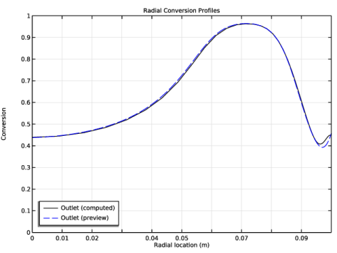
Clear the Additional parallel lines checkbox.
Line Graph 1
1
In the Model Builder window, expand the Temperature, 1D node, then click Line Graph 1.
2
In the Settings window for Line Graph, click to expand the Legends section.
3
Grid 1D 2
1
In the Results toolbar, click  More Datasets and choose Grid > Grid 1D.
2
In the Settings window for Grid 1D, locate the Parameter Bounds section.
3
In the Name text field, type x1.
4
In the Maximum text field, type 0.1.
5
Locate the Data section. From the Source list, choose Function.
6
From the Function list, choose Deep Neural Network 1 (dnn1_1, dnn1_2).
Line Graph 2
1
In the Model Builder window, right-click Temperature, 1D and choose Line Graph.
2
In the Settings window for Line Graph, locate the Data section.
3
From the Dataset list, choose Grid 1D 2.
4
Locate the y-Axis Data section. In the Expression text field, type dnn1_1(x1,L,E,ke,dHrx).
5
Locate the Legends section. Select the Show legends checkbox.
6
From the Legends list, choose Manual.
7
8
Click to expand the Coloring and Style section. Find the Line style subsection. From the Line list, choose Dashed.
9
From the Color list, choose Blue.
Temperature, 1D
1
In the Model Builder window, click Temperature, 1D.
2
In the Temperature, 1D toolbar, click  Plot.
Compare with Figure 7.
Radial Conversion Profiles
1
In the Model Builder window, expand the Results > Conversion, 1D node, then click Conversion, 1D.
2
In the Settings window for 1D Plot Group, type Radial Conversion Profiles in the Label text field.
3
Locate the Axis section. Select the Manual axis limits checkbox.
4
In the x minimum text field, type 0.
5
In the x maximum text field, type 0.1.
6
In the y minimum text field, type 0.
7
In the y maximum text field, type 1.
8
Locate the Legend section. From the Position list, choose Lower left.
9
In the Radial Conversion Profiles toolbar, click  Plot.
Compare with Figure 8.
Line Graph 1
1
In the Model Builder window, expand the Radial Conversion Profiles node, then click Line Graph 1.
2
In the Settings window for Line Graph, locate the Legends section.
3
4
Click  Delete twice.
5
Line Graph 2
1
In the Model Builder window, right-click Radial Conversion Profiles and choose Line Graph.
2
In the Settings window for Line Graph, locate the Data section.
3
From the Dataset list, choose Grid 1D 2.
4
Locate the y-Axis Data section. In the Expression text field, type dnn1_2(x1,L,E,ke,dHrx).
5
Locate the Coloring and Style section. Find the Line style subsection. From the Line list, choose Dashed.
6
From the Color list, choose Blue.
7
Locate the Legends section. Select the Show legends checkbox.
8
From the Legends list, choose Manual.
9
Radial Conversion Profiles
1
In the Model Builder window, click Radial Conversion Profiles.
2
In the Settings window for 1D Plot Group, click to expand the Title section.
3
In the Title text area, type Radial Conversion Profiles.
4
Locate the Axis section. Select the Manual axis limits checkbox.
5
In the x minimum text field, type 0.
6
In the x maximum text field, type 0.1.
7
In the y minimum text field, type 0.
8
In the y maximum text field, type 1.
9
Locate the Legend section. From the Position list, choose Lower left.
10
In the Radial Conversion Profiles toolbar, click  Plot.
Compare with Figure 7.
Finally, change the plot titles to more easily identify the surrogate model plots (preview plots) from the computed plots.
Temperature, 3D (Revolved)
1
In the Model Builder window, click Temperature, 3D (Revolved).
2
In the Settings window for 3D Plot Group, locate the Plot Settings section.
3
Clear the Plot dataset edges checkbox.
4
Click to expand the Title section. From the Title type list, choose Manual.
5
In the Title text area, type Surface: Temperature (K) (Computed).
6
Click the  Zoom Extents button in the Graphics toolbar.
7
In the Temperature, 3D (Revolved) toolbar, click  Plot.
Temperature, 3D, Surrogate (Revolved)
1
In the Model Builder window, click Temperature, 3D, Surrogate (Revolved).
2
In the Settings window for 3D Plot Group, locate the Title section.
3
From the Title type list, choose Manual.
4
In the Title text area, type Surface: Temperature (K) (Preview).
Conversion, 3D (Revolved )
1
In the Model Builder window, click Conversion, 3D (Revolved ).
2
In the Settings window for 3D Plot Group, locate the Plot Settings section.
3
Clear the Plot dataset edges checkbox.
4
Locate the Title section. From the Title type list, choose Manual.
5
In the Title text area, type Surface: Conversion, species A (Computed).
Conversion, 30, Surrogate
1
In the Model Builder window, click Conversion, 30, Surrogate.
2
In the Settings window for 3D Plot Group, locate the Title section.
3
From the Title type list, choose Manual.
4
In the Title text area, type Surface: Conversion, species A (Preview).