PDF

Beam with a Traveling Load
Introduction
In some problems, the load changes position with time. It can be a train moving over a bridge or a heat source moving along a weld. In this example, intended to show how to model traveling loads, a set of load pulses travel along a beam with equally spaced supports.
The model is parameterized, so it is easy to change, for example, the velocity of the load pulses or the spacing between them. This is used for showing that for some load configurations, resonant vibrations will appear in the beam.
Modeling traveling loads
The possibility to enter analytical expressions and use built-in or external functions in the input fields for loads and boundary conditions makes it easy model traveling loads in COMSOL Multiphysics. A load with a constant distribution moving with a constant velocity v can mathematically be written
(1)
This is the type of load being used in this example. You can, however, use completely arbitrary functions of space and time.
When the load is moving during the analysis, it will in general only cover some elements partially. This is not a problem, since the load is numerically integrated. The element size should, however, be chosen such that several elements are covered by the load.
Model Definition
Geometry
Many aspects of the modeling can be parameterized. Table 1 below shows the values used in the analysis.
Material Properties and Boundary Conditions
The material is concrete, with material data taken from the Material Library:
Young’s modulus E = 25 GPa
Mass density ρ = 2300 kg/m3
The beam is supported on one point at the end of each span.
The load travels along the top. The loading is controlled by the parameters listed in Table 2.
As can be seen in the table, four different combinations of loads are analyzed:
1
2
3
4
Results
The lowest eigenfrequency of the beam can be computed analytically and is independent of the number of spans. It is actually the same as for a simply supported beam with the length of a single span. The expression is
(2)
which with the given parameters can be evaluated to 4.49 Hz. It can thus be expected that a load that travels one span Ls during half the period T0 of the lowest natural frequency f0 should be able to excite a resonant vibration. This critical velocity is then approximately
(3)
The effect of changing the velocity of the load and the spacing between the loads is shown in Figure 1. The graphs show how the vertical displacement at the midpoint of the first span vary as function of the position of the first load pulse. The horizontal axis can also be seen as time, scaled with load velocity.
From the graphs, is can be seen that
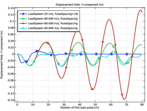
At a low load speed (20 m/s), the solution resembles a stationary solution. As the load moves away from the first span, the deflection there decreases.
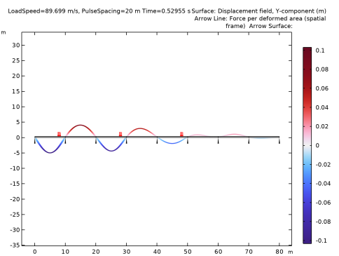
When the load speed is such (89.7 m/s) that the load travels two spans in the time T0 of one period, then the load can actually excite resonances. This can be seen when using a very long load spacing (160 m, essentially giving a single load), as well as when using a spacing of two spans (20 m). The reason is that the load will always act on a downward motion of the beam, thus giving a positive power input.
Figure 1: Displacement history at the midpoint of the first span, as function of the location of the first load pulse.
Figure 2: Displaced shape when loads are traveling to the right with a speed and spacing giving an amplification of the response.
Application Library path: COMSOL_Multiphysics/Structural_Mechanics/traveling_load
Modeling Instructions
From the File menu, choose New.
New
In the New window, click  Model Wizard.
Model Wizard
1
In the Model Wizard window, click  2D.
2
In the Select Physics tree, select Structural Mechanics > Solid Mechanics (solid).
3
Click Add.
4
Click  Study.
5
In the Select Study tree, select General Studies > Time Dependent.
6
Global Definitions
Parameters 1
1
In the Model Builder window, under Global Definitions click Parameters 1.
2
In the Settings window for Parameters, locate the Parameters section.
3
Click  Load from File.
4
Geometry 1
Rectangle 1 (r1)
1
In the Geometry toolbar, click  Rectangle.
2
In the Settings window for Rectangle, locate the Size and Shape section.
3
In the Width text field, type SpanWidth.
4
In the Height text field, type BeamHeight.
Point 1 (pt1)
1
In the Geometry toolbar, click  Point.
2
In the Settings window for Point, locate the Point section.
3
In the y text field, type BeamHeight/2.
Point 2 (pt2)
1
Right-click Point 1 (pt1) and choose Duplicate.
2
In the Settings window for Point, locate the Point section.
3
In the x text field, type SpanWidth.
4
Click  Build All Objects.
Union 1 (uni1)
1
In the Geometry toolbar, click  Booleans and Partitions and choose Union.
2
Click in the Graphics window and then press Ctrl+A to select all objects.
3
In the Settings window for Union, click  Build Selected.
Array 1 (arr1)
1
In the Geometry toolbar, click  Transforms and choose Array.
2
3
In the Settings window for Array, locate the Size section.
4
In the x size text field, type NumSpans.
5
Locate the Displacement section. In the x text field, type SpanWidth.
6
Click  Build All Objects.
7
Click the  Zoom Extents button in the Graphics toolbar.
Definitions
Box: Points on Centerline
1
In the Definitions toolbar, click  Box.
2
In the Settings window for Box, type Box: Points on Centerline in the Label text field.
3
Locate the Geometric Entity Level section. From the Level list, choose Point.
4
Locate the Box Limits section. In the y minimum text field, type BeamHeight/3.
5
In the y maximum text field, type 2*BeamHeight/3.
6
Locate the Output Entities section. From the Include entity if list, choose Entity inside box.
Box: Boundaries Above
1
In the Definitions toolbar, click  Box.
2
In the Settings window for Box, type Box: Boundaries Above in the Label text field.
3
Locate the Geometric Entity Level section. From the Level list, choose Boundary.
4
Locate the Box Limits section. In the y minimum text field, type 2*BeamHeight/2.
5
Locate the Output Entities section. From the Include entity if list, choose Entity inside box.
Add Material
1
In the Materials toolbar, click  Add Material to open the Add Material window.
2
Go to the Add Material window.
3
In the tree, select Built-in > Concrete.
4
Click the Add to Component button in the window toolbar.
5
In the Materials toolbar, click  Add Material to close the Add Material window.
Solid Mechanics (solid)
1
In the Settings window for Solid Mechanics, locate the 2D Approximation section.
2
Linear Elastic Material 1
In the Model Builder window, under Component 1 (comp1) > Solid Mechanics (solid) click Linear Elastic Material 1.
Damping 1
1
In the Physics toolbar, click  Attributes and choose Damping.
2
In the Settings window for Damping, locate the Damping Settings section.
3
In the βdK text field, type 0.002.
Fixed Constraint 1
1
In the Physics toolbar, click  Points and choose Fixed Constraint.
2
In the Settings window for Fixed Constraint, locate the Point Selection section.
3
From the Selection list, choose Box: Points on Centerline.
Definitions
Create functions describing the load. The distribution is a rectangular load.
Rectangle 1 (rect1)
1
In the Definitions toolbar, click  More Functions and choose Rectangle.
2
In the Settings window for Rectangle, locate the Parameters section.
3
In the Lower limit text field, type -0.5*PulseWidth.
4
In the Upper limit text field, type 0.5*PulseWidth.
5
Click to expand the Smoothing section. In the Size of transition zone text field, type 0.1*PulseWidth.
In order to make the load pulse periodic, call it through an analytical function, which has the option of being periodic.
Analytic 1 (an1)
1
In the Definitions toolbar, click  Analytic.
2
In the Settings window for Analytic, type Pulse in the Function name text field.
3
Locate the Definition section. In the Expression text field, type rect1(x).
4
Locate the Units section. In the table, enter the following settings:
5
In the Function text field, type 1.
6
Click to expand the Periodic Extension section. Select the Make periodic checkbox.
7
In the Upper limit text field, type PulseSpacing.
Variables 1
1
In the Model Builder window, right-click Definitions and choose Variables.
Create a variable for filtering the load, so that it is periodic only behind the first pulse.
2
In the Settings window for Variables, locate the Variables section.
3
Add the load definition to the whole upper boundary. The function call will make the load nonzero only at certain traveling positions.
Solid Mechanics (solid)
Boundary Load 1
1
In the Physics toolbar, click  Boundaries and choose Boundary Load.
2
In the Settings window for Boundary Load, locate the Boundary Selection section.
3
From the Selection list, choose Box: Boundaries Above.
4
Locate the Force section. Specify the fA vector as
Mesh 1
Mapped 1
In the Mesh toolbar, click  Mapped.
Distribution 1
1
Right-click Mapped 1 and choose Distribution.
2
3
In the Settings window for Distribution, locate the Distribution section.
4
In the Number of elements text field, type 1.
Distribution 2
1
In the Model Builder window, right-click Mapped 1 and choose Distribution.
2
In the Settings window for Distribution, locate the Boundary Selection section.
3
From the Selection list, choose Box: Boundaries Above.
4
Locate the Distribution section. In the Number of elements text field, type ElemPerSpan.
5
Click  Build All.
Add a parametric sweep to study the four load pulse scenarios.
Study 1
Parametric Sweep
1
In the Study toolbar, click  Parametric Sweep.
2
In the Settings window for Parametric Sweep, locate the Study Settings section.
3
4
5
Step 1: Time Dependent
1
In the Model Builder window, click Step 1: Time Dependent.
2
In the Settings window for Time Dependent, locate the Study Settings section.
3
In the Output times text field, type range(0,SpanWidth/LoadSpeed/20,Tend).
4
From the Tolerance list, choose User controlled.
5
In the Relative tolerance text field, type 0.0001.
Solution 1 (sol1)
1
In the Study toolbar, click  Show Default Solver.
2
In the Model Builder window, expand the Solution 1 (sol1) node, then click Time-Dependent Solver 1.
3
In the Settings window for Time-Dependent Solver, click to expand the Time Stepping section.
4
From the Maximum step constraint list, choose Constant.
5
In the Maximum step text field, type Tstep.
Set a reasonable scale for the displacements, so that the convergence checks in the solver will be appropriate.
6
In the Model Builder window, expand the Study 1 > Solver Configurations > Solution 1 (sol1) > Dependent Variables 1 node, then click Displacement Field (comp1.u).
7
In the Settings window for Field, locate the Scaling section.
8
In the Scale text field, type 1e-2.
Run the parametric sweep containing four time dependent studies.
9
In the Study toolbar, click  Compute.
Results
Displacement
In the Settings window for 2D Plot Group, type Displacement in the Label text field.
Surface 1
1
In the Model Builder window, expand the Displacement node, then click Surface 1.
2
In the Settings window for Surface, locate the Expression section.
3
In the Expression text field, type v.
4
Locate the Coloring and Style section. From the Color table list, choose Wave.
5
From the Scale list, choose Linear symmetric.
Deformation
1
In the Model Builder window, expand the Surface 1 node, then click Deformation.
2
In the Settings window for Deformation, locate the Scale section.
3
Select the Scale factor checkbox. In the associated text field, type 50.
Modify the predefined load plot and add it on top of the displacement plot.
Result Templates
1
In the Results toolbar, click  Result Templates to open the Result Templates window.
2
Go to the Result Templates window.
3
In the tree, select Study 1/Parametric Solutions 1 (sol2) > Solid Mechanics > Applied Loads (solid) > Boundary Loads (solid).
4
Click the Add Result Template button in the window toolbar.
5
In the Results toolbar, click  Result Templates to close the Result Templates window.
Results
Load Arrows
1
In the Model Builder window, expand the Results > Boundary Loads (solid) node, then click Boundary Load 1.
2
In the Settings window for Arrow Line, type Load Arrows in the Label text field.
3
Locate the Arrow Positioning section. From the Placement list, choose Uniform.
4
In the Number of arrows text field, type 1000.
5
Locate the Coloring and Style section. From the Arrow base list, choose Head.
6
Select the Scale factor checkbox. In the associated text field, type 1.5e-5.
7
In the Boundary Loads (solid) toolbar, click  Plot.
8
In the Model Builder window, expand the Load Arrows node.
Color Expression, Deformation
1
In the Model Builder window, under Results > Boundary Loads (solid) > Load Arrows, Ctrl-click to select Color Expression and Deformation.
2
Load Arrows
Right-click Results > Boundary Loads (solid) > Load Arrows and choose Copy.
Load Arrows
In the Model Builder window, right-click Displacement and choose Paste Arrow Line.
Boundary Loads (solid)
In the Model Builder window, under Results right-click Boundary Loads (solid) and choose Delete.
Supports
1
In the Model Builder window, right-click Displacement and choose Arrow Surface.
Add a visualization of the supports.
2
In the Settings window for Arrow Surface, type Supports in the Label text field.
3
Locate the Expression section. In the X-component text field, type 0.
4
In the Y-component text field, type 1.
5
Locate the Arrow Positioning section. Find the X grid points subsection. From the Entry method list, choose Coordinates.
6
In the Coordinates text field, type range(0,SpanWidth,TotLength).
7
Find the Y grid points subsection. From the Entry method list, choose Coordinates.
8
In the Coordinates text field, type 0.
9
Locate the Coloring and Style section. From the Arrow type list, choose Cone.
10
From the Arrow base list, choose Head.
11
Select the Scale factor checkbox. In the associated text field, type 2.
12
From the Color list, choose Black.
Displacement
1
In the Model Builder window, click Displacement.
2
In the Settings window for 2D Plot Group, locate the Data section.
3
From the Time (s) list, choose 0.52955.
4
In the Displacement toolbar, click  Plot.
5
From the Parameter value (LoadSpeed (m/s),PulseSpacing (m)) list, choose 3: LoadSpeed=89.699 m/s, PulseSpacing=20 m.
6
In the Displacement toolbar, click  Plot.
7
Click the  Zoom Extents button in the Graphics toolbar.
Animate the four different cases.
Animation 1
1
In the Displacement toolbar, click  Animation and choose Player.
2
In the Settings window for Animation, locate the Animation Editing section.
3
From the Parameter value (LoadSpeed (m/s),PulseSpacing (m)) list, choose 2: LoadSpeed=89.699 m/s, PulseSpacing=160 m.
4
Click the  Play button in the Graphics toolbar.
5
From the Parameter value (LoadSpeed (m/s),PulseSpacing (m)) list, choose 3: LoadSpeed=89.699 m/s, PulseSpacing=20 m.
6
Click the  Play button in the Graphics toolbar.
7
From the Parameter value (LoadSpeed (m/s),PulseSpacing (m)) list, choose 4: LoadSpeed=89.699 m/s, PulseSpacing=10 m.
8
Click the  Play button in the Graphics toolbar.
Create a point at the midpoint of the first span. This is where the vertical displacement will be compared between the four cases.
Cut Point 2D 1
1
In the Results toolbar, click  Cut Point 2D.
2
In the Settings window for Cut Point 2D, locate the Point Data section.
3
In the X text field, type SpanWidth/2.
4
In the Y text field, type BeamHeight/2.
5
Locate the Data section. From the Dataset list, choose Study 1/Parametric Solutions 1 (sol2).
1D Plot Group 2
In the Results toolbar, click  1D Plot Group.
Point Graph 1
1
Right-click 1D Plot Group 2 and choose Point Graph.
2
In the Settings window for Point Graph, locate the Data section.
3
From the Dataset list, choose Cut Point 2D 1.
4
Locate the y-Axis Data section. In the Expression text field, type v.
5
In the 1D Plot Group 2 toolbar, click  Plot.
Since the time spans are different for different load speeds, it is more informative to study the results versus the position of the first load pulse.
6
Locate the x-Axis Data section. From the Parameter list, choose Expression.
7
In the Expression text field, type t*LoadSpeed.
8
Click to expand the Coloring and Style section. From the Width list, choose 2.
9
Find the Line markers subsection. From the Marker list, choose Cycle.
10
From the Positioning list, choose Interpolated.
11
Click to expand the Legends section. Select the Show legends checkbox.
12
In the 1D Plot Group 2 toolbar, click  Plot.
1D Plot Group 2
1
In the Model Builder window, click 1D Plot Group 2.
2
In the Settings window for 1D Plot Group, locate the Legend section.
3
From the Position list, choose Upper left.
4
Locate the Plot Settings section.
5
Select the x-axis label checkbox. In the associated text field, type Position of first load pulse [m].
6
In the 1D Plot Group 2 toolbar, click  Plot.