|
|
•
|
|
1
|
|
2
|
|
3
|
Click Add.
|
|
4
|
|
5
|
Click
|
|
1
|
|
2
|
|
3
|
|
4
|
|
1
|
|
2
|
|
3
|
|
4
|
|
5
|
|
6
|
|
7
|
Locate the Selections of Resulting Entities section. Select the Resulting objects selection checkbox.
|
|
1
|
|
2
|
|
3
|
|
4
|
|
5
|
Locate the Selections of Resulting Entities section. Select the Resulting objects selection checkbox.
|
|
1
|
|
2
|
|
3
|
|
4
|
|
1
|
Go to the Add Material window.
|
|
2
|
|
3
|
Click the Add to Component button in the window toolbar.
|
|
4
|
|
1
|
|
2
|
|
1
|
|
2
|
In the Show More Options dialog, in the tree, select the checkbox for the node Study > Reduced-Order Modeling.
|
|
3
|
Click OK.
|
|
1
|
|
2
|
|
1
|
In the Model Builder window, under Component 1: Physics (comp1) > Heat Equation (hteq) click Heat Equation 1.
|
|
2
|
|
3
|
|
4
|
|
5
|
Locate the Damping or Mass Coefficient section. In the da text field, type mat1.def.rho*mat1.def.Cp.
|
|
1
|
|
2
|
|
3
|
|
1
|
|
3
|
|
4
|
|
5
|
|
1
|
|
3
|
|
4
|
|
1
|
|
2
|
|
3
|
|
4
|
|
5
|
|
1
|
|
2
|
In the Settings window for Point Probe, type Thermostat position 2: Full Model in the Label text field.
|
|
3
|
|
4
|
|
1
|
In the Model Builder window, under Component 1: Physics (comp1) > Definitions, Ctrl-click to select Thermostat position 1: Full Model (ppb1) and Thermostat position 2: Full Model (ppb2).
|
|
2
|
Right-click and choose Group.
|
|
1
|
In the Model Builder window, under Component 2: Controller Events (comp2) right-click Definitions and choose Variables.
|
|
2
|
|
4
|
|
1
|
|
2
|
Go to the Add Study window.
|
|
3
|
|
4
|
Click the Add Study button in the window toolbar.
|
|
5
|
|
1
|
In the Settings window for Study, type Study 1: Model Reduction with 6 Modes in the Label text field.
|
|
2
|
|
3
|
Clear the Generate convergence plots checkbox.
|
|
1
|
|
2
|
|
3
|
Select the Desired number of eigenvalues checkbox.
|
|
4
|
|
1
|
|
2
|
|
3
|
|
4
|
|
1
|
|
2
|
|
3
|
|
4
|
|
5
|
|
6
|
Locate the Outputs section. In the table, enter the following settings:
|
|
7
|
Locate the Model Control Inputs section. In the table, set up the training values: change the value of Tout to 293.15 and HeatState to 1.
|
|
8
|
|
9
|
|
1
|
|
2
|
Go to the Add Physics window.
|
|
3
|
|
4
|
Click the Add to Component 2: Controller Events button in the window toolbar.
|
|
5
|
|
1
|
|
2
|
|
1
|
|
2
|
|
1
|
|
2
|
|
3
|
|
4
|
Clear the Use consistent initialization checkbox.
|
|
5
|
Locate the Reinitialization section. In the table, enter the following settings:
|
|
1
|
|
2
|
|
3
|
|
4
|
Clear the Use consistent initialization checkbox.
|
|
5
|
Locate the Reinitialization section. In the table, enter the following settings:
|
|
1
|
In the Model Builder window, under Global Definitions > Reduced-Order Modeling click Global Reduced-Model Inputs 1.
|
|
2
|
|
1
|
In the Model Builder window, under Study 1: Model Reduction with 6 Modes > Step 2: Model Reduction click Time Dependent 1.
|
|
2
|
|
3
|
In the Solve for column of the table, clear the checkbox for Component 2: Controller Events (comp2).
|
|
1
|
|
2
|
Go to the Add Study window.
|
|
3
|
|
4
|
Click the Add Study button in the window toolbar.
|
|
5
|
|
1
|
|
2
|
|
3
|
|
4
|
|
5
|
|
6
|
|
7
|
Clear the Generate convergence plots checkbox.
|
|
1
|
|
2
|
|
3
|
Click
|
|
5
|
|
1
|
|
2
|
|
3
|
In the Model Builder window, under Study 2: Controller Full > Solver Configurations > Solution 3 (sol3) click Time-Dependent Solver 1.
|
|
4
|
|
5
|
|
6
|
|
1
|
|
2
|
|
3
|
Select the Modify model configuration for study step checkbox.
|
|
4
|
In the tree, select Global Definitions > Reduced-Order Modeling > Time Dependent, Modal Reduced-Order Model 1 (rom1).
|
|
5
|
Right-click and choose Disable.
|
|
6
|
|
1
|
|
2
|
|
3
|
|
4
|
|
1
|
|
2
|
|
3
|
|
4
|
|
1
|
In the Model Builder window, under Component 1: Physics (comp1) > Definitions, Ctrl-click to select Thermostat position 1: Reduced Model 1 (var1) and Thermostat position 2: Reduced Model 1 (var2).
|
|
2
|
Right-click and choose Group.
|
|
1
|
In the Model Builder window, under Component 2: Controller Events (comp2) right-click Definitions and choose Variables.
|
|
2
|
|
4
|
In the Label text field, type Variables 2: Temperature at Position 1 or 2 Using the Reduced Model 1.
|
|
1
|
|
2
|
|
3
|
In the tree, select Component 2: Controller Events (comp2) > Definitions > Variables 2: Temperature at Position 1 or 2 Using the Reduced Model 1.
|
|
4
|
Right-click and choose Disable.
|
|
1
|
|
2
|
Go to the Add Study window.
|
|
3
|
|
4
|
Click the Add Study button in the window toolbar.
|
|
5
|
|
1
|
|
2
|
Clear the Generate default plots checkbox.
|
|
3
|
Clear the Generate convergence plots checkbox.
|
|
4
|
|
5
|
|
1
|
|
2
|
In the Solve for column of the table, under Component 1: Physics (comp1), clear the checkbox for Heat Equation (hteq).
|
|
3
|
|
4
|
|
5
|
Locate the Physics and Variables Selection section. Select the Modify model configuration for study step checkbox.
|
|
6
|
In the tree, select Component 2: Controller Events (comp2) > Definitions > Variables 1: Temperature at Position 1 or 2 Using the Full Model.
|
|
7
|
Right-click and choose Disable.
|
|
8
|
|
9
|
In the Probes list, choose Thermostat position 1: Full Model (ppb1) and Thermostat position 2: Full Model (ppb2).
|
|
10
|
|
1
|
|
2
|
|
3
|
Click
|
|
5
|
|
1
|
|
2
|
|
3
|
In the Model Builder window, under Study 3: Controller ROM with 6 Modes > Solver Configurations > Solution 7 (sol7) click Time-Dependent Solver 1.
|
|
4
|
|
5
|
|
6
|
|
7
|
|
1
|
|
2
|
|
3
|
|
4
|
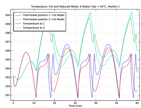
In the Label text field, type Temperature: Full and Reduced Model, 6 Modes, Tset = 20°C, Position 1.
|
|
5
|
|
6
|
|
7
|
|
1
|
Right-click Temperature: Full and Reduced Model, 6 Modes, Tset = 20°C, Position 1 and choose Global.
|
|
2
|
|
3
|
|
4
|
|
5
|
|
6
|
Locate the y-Axis Data section. In the table, enter the following settings:
|
|
7
|
|
8
|
|
9
|
|
1
|
In the Model Builder window, right-click Temperature: Full and Reduced Model, 6 Modes, Tset = 20°C, Position 1 and choose Global.
|
|
2
|
In the Settings window for Global, type Temperature: Reduced Model with 6 Modes in the Label text field.
|
|
3
|
Locate the Data section. From the Dataset list, choose Study 3: Controller ROM with 6 Modes/Parametric Solutions 2 (11) (sol8).
|
|
4
|
|
5
|
|
6
|
Locate the y-Axis Data section. In the table, enter the following settings:
|
|
7
|
|
8
|
|
9
|
|
1
|
Right-click Temperature: Full and Reduced Model, 6 Modes, Tset = 20°C, Position 1 and choose Duplicate.
|
|
2
|
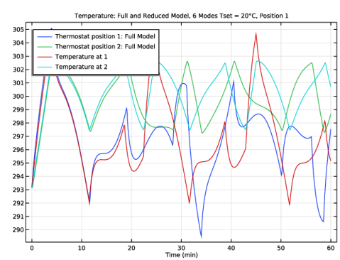
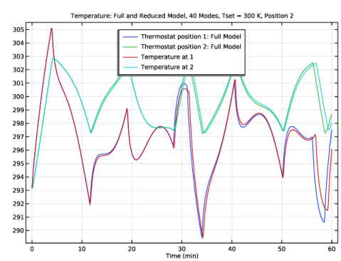
In the Settings window for 1D Plot Group, type Temperature: Full and Reduced Model, 6 Modes, Tset = 300 K, Position 2 in the Label text field.
|
|
1
|
In the Model Builder window, expand the Temperature: Full and Reduced Model, 6 Modes, Tset = 300 K, Position 2 node, then click Temperature: Full Model.
|
|
2
|
|
3
|
|
1
|
|
2
|
|
3
|
|
4
|
|
1
|
In the Model Builder window, click Temperature: Full and Reduced Model, 6 Modes, Tset = 300 K, Position 2.
|
|
2
|
|
3
|
|
1
|
|
2
|
Go to the Add Study window.
|
|
3
|
|
4
|
Click the Add Study button in the window toolbar.
|
|
5
|
|
1
|
In the Settings window for Study, type Study 4: Model Reduction with 40 Modes in the Label text field.
|
|
2
|
|
3
|
Clear the Generate convergence plots checkbox.
|
|
1
|
|
2
|
|
3
|
|
1
|
|
2
|
|
3
|
|
4
|
|
1
|
|
2
|
|
3
|
|
4
|
|
5
|
|
6
|
Locate the Outputs section. In the table, enter the following settings:
|
|
7
|
Locate the Model Control Inputs section. In the table, set up the training values: change the value of Tout to 293.15 and HeatState to 1.
|
|
8
|
|
1
|
|
2
|
|
3
|
Select the Modify model configuration for study step checkbox.
|
|
4
|
In the tree, select Global Definitions > Reduced-Order Modeling > Time Dependent, Modal Reduced-Order Model 1 (rom1).
|
|
5
|
Right-click and choose Disable.
|
|
6
|
In the tree, select Component 2: Controller Events (comp2) > Definitions > Variables 1: Temperature at Position 1 or 2 Using the Full Model and Component 2: Controller Events (comp2) > Definitions > Variables 2: Temperature at Position 1 or 2 Using the Reduced Model 1.
|
|
7
|
Right-click and choose Disable.
|
|
8
|
|
1
|
In the Model Builder window, under Study 4: Model Reduction with 40 Modes > Step 2: Model Reduction click Time Dependent 1.
|
|
2
|
|
3
|
Select the Modify model configuration for study step checkbox.
|
|
4
|
In the tree, select Global Definitions > Reduced-Order Modeling > Time Dependent, Modal Reduced-Order Model 1 (rom1).
|
|
5
|
Right-click and choose Disable.
|
|
6
|
In the tree, select Component 2: Controller Events (comp2).
|
|
7
|
Right-click and choose Disable in Solvers.
|
|
8
|
In the tree, select Component 2: Controller Events (comp2) > Definitions > Variables 1: Temperature at Position 1 or 2 Using the Full Model and Component 2: Controller Events (comp2) > Definitions > Variables 2: Temperature at Position 1 or 2 Using the Reduced Model 1.
|
|
9
|
Right-click and choose Disable.
|
|
10
|
|
1
|
In the Model Builder window, under Global Definitions > Reduced-Order Modeling click Time Dependent, Modal Reduced-Order Model 1 (rom1).
|
|
2
|
In the Settings window for Time Dependent, Modal Reduced-Order Model, type Time Dependent, Modal Reduced-Order Model 1: 6 Modes in the Label text field.
|
|
1
|
In the Model Builder window, under Global Definitions > Reduced-Order Modeling click Time Dependent, Modal Reduced-Order Model 2 (rom2).
|
|
2
|
In the Settings window for Time Dependent, Modal Reduced-Order Model, type Time Dependent, Modal Reduced-Order Model 2: 40 Modes in the Label text field.
|
|
1
|
|
2
|
In the Settings window for Global Variable Probe, type Thermostat Position 1: Reduced Model 2 in the Label text field.
|
|
3
|
|
1
|
|
2
|
In the Settings window for Global Variable Probe, type Thermostat Position 2: Reduced Model 2 in the Label text field.
|
|
3
|
|
1
|
In the Model Builder window, under Component 1: Physics (comp1) > Definitions, Ctrl-click to select Thermostat Position 1: Reduced Model 2 (var3) and Thermostat Position 2: Reduced Model 2 (var4).
|
|
2
|
Right-click and choose Group.
|
|
1
|
In the Model Builder window, under Component 2: Controller Events (comp2) right-click Definitions and choose Variables.
|
|
2
|
In the Settings window for Variables, type Variables 3: Temperature at Position 1 or 2 Using the Reduced Model 2 in the Label text field.
|
|
3
|
Locate the Variables section. In the table, enter the following settings:
|
|
1
|
|
2
|
|
3
|
Select the Modify model configuration for study step checkbox.
|
|
4
|
In the tree, select Component 2: Controller Events (comp2) > Definitions > Variables 1: Temperature at Position 1 or 2 Using the Full Model, Component 2: Controller Events (comp2) > Definitions > Variables 2: Temperature at Position 1 or 2 Using the Reduced Model 1, and Component 2: Controller Events (comp2) > Definitions > Variables 3: Temperature at Position 1 or 2 Using the Reduced Model 2.
|
|
5
|
Right-click and choose Disable.
|
|
6
|
In the tree, select Global Definitions > Reduced-Order Modeling > Time Dependent, Modal Reduced-Order Model 1: 6 Modes (rom1) and Global Definitions > Reduced-Order Modeling > Time Dependent, Modal Reduced-Order Model 2: 40 Modes (rom2).
|
|
7
|
Right-click and choose Disable.
|
|
1
|
In the Model Builder window, under Study 1: Model Reduction with 6 Modes > Step 2: Model Reduction click Time Dependent 1.
|
|
2
|
|
3
|
Select the Modify model configuration for study step checkbox.
|
|
4
|
In the tree, select Component 2: Controller Events (comp2) > Definitions > Variables 1: Temperature at Position 1 or 2 Using the Full Model, Component 2: Controller Events (comp2) > Definitions > Variables 2: Temperature at Position 1 or 2 Using the Reduced Model 1, and Component 2: Controller Events (comp2) > Definitions > Variables 3: Temperature at Position 1 or 2 Using the Reduced Model 2.
|
|
5
|
Right-click and choose Disable.
|
|
6
|
In the tree, select Global Definitions > Reduced-Order Modeling > Time Dependent, Modal Reduced-Order Model 1: 6 Modes (rom1), Global Definitions > Reduced-Order Modeling > Time Dependent, Modal Reduced-Order Model 2: 40 Modes (rom2), Component 2: Controller Events (comp2) > Definitions > Variables 1: Temperature at Position 1 or 2 Using the Full Model, Component 2: Controller Events (comp2) > Definitions > Variables 2: Temperature at Position 1 or 2 Using the Reduced Model 1, and Component 2: Controller Events (comp2) > Definitions > Variables 3: Temperature at Position 1 or 2 Using the Reduced Model 2.
|
|
7
|
Right-click and choose Disable.
|
|
1
|
|
2
|
|
3
|
In the tree, select Global Definitions > Reduced-Order Modeling > Time Dependent, Modal Reduced-Order Model 2: 40 Modes (rom2).
|
|
4
|
Right-click and choose Disable.
|
|
5
|
In the tree, select Global Definitions > Reduced-Order Modeling > Time Dependent, Modal Reduced-Order Model 2: 40 Modes (rom2) and Component 2: Controller Events (comp2) > Definitions > Variables 3: Temperature at Position 1 or 2 Using the Reduced Model 2.
|
|
6
|
Right-click and choose Disable.
|
|
7
|
|
8
|
In the Probes list, choose Thermostat position 1: Reduced Model 1 (var1), Thermostat position 2: Reduced Model 1 (var2), Thermostat Position 1: Reduced Model 2 (var3), and Thermostat Position 2: Reduced Model 2 (var4).
|
|
9
|
|
1
|
In the Model Builder window, under Study 3: Controller ROM with 6 Modes click Step 1: Time Dependent.
|
|
2
|
|
3
|
In the tree, select Global Definitions > Reduced-Order Modeling > Time Dependent, Modal Reduced-Order Model 2: 40 Modes (rom2).
|
|
4
|
Right-click and choose Disable.
|
|
5
|
In the tree, select Component 2: Controller Events (comp2) > Definitions > Variables 3: Temperature at Position 1 or 2 Using the Reduced Model 2.
|
|
6
|
Right-click and choose Disable.
|
|
7
|
Locate the Results While Solving section. In the Probes list, choose Thermostat Position 1: Reduced Model 2 (var3) and Thermostat Position 2: Reduced Model 2 (var4).
|
|
8
|
|
1
|
|
2
|
|
3
|
In the tree, select Global Definitions > Reduced-Order Modeling > Time Dependent, Modal Reduced-Order Model 1: 6 Modes (rom1) and Global Definitions > Reduced-Order Modeling > Time Dependent, Modal Reduced-Order Model 2: 40 Modes (rom2).
|
|
4
|
Right-click and choose Disable.
|
|
5
|
In the tree, select Component 2: Controller Events (comp2) > Definitions > Variables 3: Temperature at Position 1 or 2 Using the Reduced Model 2.
|
|
6
|
Right-click and choose Disable.
|
|
1
|
In the Model Builder window, under Study 4: Model Reduction with 40 Modes > Step 2: Model Reduction click Time Dependent 1.
|
|
2
|
|
3
|
In the tree, select Global Definitions > Reduced-Order Modeling > Time Dependent, Modal Reduced-Order Model 1: 6 Modes (rom1), Global Definitions > Reduced-Order Modeling > Time Dependent, Modal Reduced-Order Model 2: 40 Modes (rom2), Component 2: Controller Events (comp2) > Definitions > Variables 1: Temperature at Position 1 or 2 Using the Full Model, Component 2: Controller Events (comp2) > Definitions > Variables 2: Temperature at Position 1 or 2 Using the Reduced Model 1, and Component 2: Controller Events (comp2) > Definitions > Variables 3: Temperature at Position 1 or 2 Using the Reduced Model 2.
|
|
4
|
Right-click and choose Disable.
|
|
1
|
|
2
|
Go to the Add Study window.
|
|
3
|
|
4
|
Click the Add Study button in the window toolbar.
|
|
5
|
|
1
|
In the Settings window for Study, type Study 5: Controller ROM with 40 Modes in the Label text field.
|
|
2
|
|
3
|
Clear the Generate convergence plots checkbox.
|
|
1
|
In the Model Builder window, under Study 5: Controller ROM with 40 Modes click Step 1: Time Dependent.
|
|
2
|
|
3
|
|
4
|
|
5
|
Locate the Physics and Variables Selection section. Select the Modify model configuration for study step checkbox.
|
|
6
|
In the tree, select Global Definitions > Reduced-Order Modeling > Time Dependent, Modal Reduced-Order Model 1: 6 Modes (rom1).
|
|
7
|
Right-click and choose Disable.
|
|
8
|
|
9
|
Right-click and choose Disable in Solvers.
|
|
10
|
In the tree, select Component 2: Controller Events (comp2) > Definitions > Variables 1: Temperature at Position 1 or 2 Using the Full Model and Component 2: Controller Events (comp2) > Definitions > Variables 2: Temperature at Position 1 or 2 Using the Reduced Model 1.
|
|
11
|
Right-click and choose Disable.
|
|
12
|
|
13
|
In the Probes list, choose Thermostat position 1: Full Model (ppb1), Thermostat position 2: Full Model (ppb2), Thermostat position 1: Reduced Model 1 (var1), and Thermostat position 2: Reduced Model 1 (var2).
|
|
14
|
|
1
|
|
2
|
|
3
|
Click
|
|
5
|
|
1
|
|
2
|
|
3
|
In the Model Builder window, under Study 5: Controller ROM with 40 Modes > Solver Configurations > Solution 13 (sol13) click Time-Dependent Solver 1.
|
|
4
|
|
5
|
|
6
|
|
7
|
|
1
|
In the Model Builder window, expand the Study 5: Controller ROM with 40 Modes > Solver Configurations > Parametric Solutions 3 (sol14) node.
|
|
2
|
Right-click Temperature: Full and Reduced Model, 6 Modes, Tset = 20°C, Position 1 and choose Duplicate.
|
|
3
|
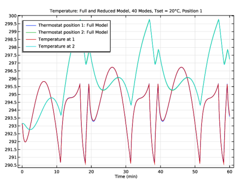
In the Settings window for 1D Plot Group, type Temperature: Full and Reduced Model, 40 Modes, Tset = 20°C, Position 1 in the Label text field.
|
|
4
|
Locate the Title section. In the Title text area, type Temperature: Full and Reduced Model, 40 Modes, Tset = 20°C, Position 1.
|
|
1
|
In the Model Builder window, expand the Temperature: Full and Reduced Model, 40 Modes, Tset = 20°C, Position 1 node, then click Temperature: Reduced Model with 6 Modes.
|
|
2
|
In the Settings window for Global, type Temperature: Reduced Model with 40 Modes in the Label text field.
|
|
3
|
Locate the Data section. From the Dataset list, choose Study 5: Controller ROM with 40 Modes/Parametric Solutions 3 (21) (sol14).
|
|
4
|
Locate the y-Axis Data section. In the table, enter the following settings:
|
|
5
|
|
1
|
In the Model Builder window, right-click Temperature: Full and Reduced Model, 6 Modes, Tset = 300 K, Position 2 and choose Duplicate.
|
|
2
|
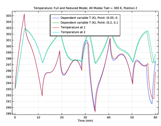
In the Settings window for 1D Plot Group, type Temperature: Full and Reduced Model, 40 Modes, Tset = 300 K, Position 2 in the Label text field.
|
|
3
|
Locate the Title section. In the Title text area, type Temperature: Full and Reduced Model, 40 Modes, Tset = 300 K, Position 2.
|
|
4
|
|
1
|
In the Model Builder window, expand the Temperature: Full and Reduced Model, 40 Modes, Tset = 300 K, Position 2 node, then click Temperature: Reduced Model with 6 Modes.
|
|
2
|
In the Settings window for Global, type Temperature: Reduced Model with 40 Modes in the Label text field.
|
|
3
|
Locate the Data section. From the Dataset list, choose Study 5: Controller ROM with 40 Modes/Parametric Solutions 3 (21) (sol14).
|
|
4
|
Locate the y-Axis Data section. In the table, enter the following settings:
|
|
5
|
|
1
|
|
2
|
Go to the Add Study window.
|
|
3
|
|
4
|
Click the Add Study button in the window toolbar.
|
|
5
|
|
1
|
|
2
|
|
3
|
Clear the Generate convergence plots checkbox.
|
|
1
|
|
2
|
|
3
|
|
4
|
|
1
|
|
2
|
|
3
|
|
1
|
|
2
|
|
3
|
|
1
|
|
2
|
|
3
|
|
1
|
|
2
|