PDF

Stresses in a Pulley
Introduction
This example contains a study of the stress distribution in a driving pulley. The analysis shows the stresses as functions of the pulley’s angular velocity.
Model Definition
Figure 1 shows the pulley under study (to the right) and the external forces applied due to the driving belt.
Figure 1: Pulley and driving belt with the external forces F1 and F2.
Here, F1 and F2 are the loads in the load side and in the slack side of the belt, respectively. The relationship between these forces is given by the capstan equation (or Eytelwein’s formula, as it is referred to in the German literature):
where μ is the coefficient of friction and β is the contact angle between the belt and the pulley. This equation is valid if a condition of impending slippage between the belt and the pulley prevails.
It is also necessary to state that the peripheral force (the force that transmits the power) is
Where R is the outer radius of the pulley and M is the applied torque. It is then possible to define F2 as
Now that you know the force in the slack side of the belt, you can derive the loads on the boundary of the pulley. In mechanics and the theory for flexible wires the following equilibrium equations appear:
where Fn is the normal component (directed inward) and Ft the tangential component (directed against the rotation) of the external forces, S is the tension force, and R is the radius.
If you apply these equations, the loads on the boundary of the pulley become
and
where θ is the angle for which the forces are calculated (see Figure 1).
Due to the rotation of the pulley, inertia loads are generated. These loads can be calculated as
where r is the radius, ω is the rotation speed, and ρ is the density.
The pulley is fixed at its inner diameter and the inertia loads are active in the entire geometry.
A parametric analysis shows how the rotational speed affects the stress distribution in the pulley. Because the power at the pulley shaft remains constant, the torque (defined as the ratio of the power by the rotational speed) decreases with increased speed. This means that with increased rotational speed, the inertial load increases while the driving-belt force decreases.
Results and Discussion
The following plots show the von Mises stress distribution inside the pulley for different rotational speeds in rpm (revolutions per minute).
As is evident from the plots, the stress distribution changes as the rotational speed increases.
Figure 2: von Mises stress distribution at n = 1000 rpm.
Figure 3: von Mises stress distribution at n = 5000 rpm.
Figure 4: von Mises stress distribution at n = 9000 rpm.
At the point (0.019, 0.054), the von Mises stress is maximal for the first rotational speed (n = 1000 rpm). The plot in Figure 5 shows how the rotational speed affects the von Mises stress at this specific point. First the stress decreases, but then the effect of the inertial loads becomes dominating and the stress begins to increase.
Figure 5: von Mises stress as function of rotational speed at point (0.019, 0.054).
Figure 6 shows the von Mises stresses in as part of the pulley. The stress field was evaluated using the accurate derivative recovery method, which makes it smoother.
Figure 6: von Mises stress in a part of the pulley evaluated using accurate derivative recovery.
In this example, dynamic effects have been ignored. In reality, it is possible that vibrations in the pulley could occur if the rotational speed coincides with natural frequencies of the pulley.
Notes About the COMSOL Implementation
When solving, adaptive mesh refinement helps to compute accurate stresses, as the stress concentration is not known in advance.
Application Library path: COMSOL_Multiphysics/Structural_Mechanics/stresses_in_pulley
Modeling Instructions
From the File menu, choose New.
New
In the New window, click  Model Wizard.
Model Wizard
1
In the Model Wizard window, click  2D.
2
In the Select Physics tree, select Structural Mechanics > Solid Mechanics (solid).
3
Click Add.
4
Click  Study.
5
In the Select Study tree, select General Studies > Stationary.
6
Geometry 1
Import the model geometry.
Import 1 (imp1)
1
In the Geometry toolbar, click  Import.
2
In the Settings window for Import, locate the Source section.
3
From the Source list, choose COMSOL Multiphysics file.
4
Click  Browse.
5
6
Click  Import.
Global Definitions
Parameters 1
1
In the Model Builder window, under Global Definitions click Parameters 1.
2
In the Settings window for Parameters, locate the Parameters section.
3
Click  Load from File.
4
Variables 1
1
In the Home toolbar, click  Variables and choose Global Variables.
2
In the Settings window for Variables, locate the Variables section.
3
Click  Load from File.
4
Materials
Define aluminum as the pulley material.
Add Material
1
In the Materials toolbar, click  Add Material to open the Add Material window.
2
Go to the Add Material window.
3
In the tree, select Built-in > Aluminum.
4
Click the Add to Component button in the window toolbar.
5
In the Materials toolbar, click  Add Material to close the Add Material window.
Definitions
Cylindrical System 2 (sys2)
In the Definitions toolbar, click  Coordinate Systems and choose Cylindrical System.
Solid Mechanics (solid)
1
In the Settings window for Solid Mechanics, locate the 2D Approximation section.
2
3
Locate the Thickness section. In the d text field, type d.
Body Load 1
1
In the Physics toolbar, click  Domains and choose Body Load.
2
3
In the Settings window for Body Load, locate the Coordinate System Selection section.
4
From the Coordinate system list, choose Cylindrical System 2 (sys2).
5
Locate the Force section. Specify the fV vector as
Prescribed Displacement 1
1
In the Physics toolbar, click  Boundaries and choose Prescribed Displacement.
2
3
In the Settings window for Prescribed Displacement, locate the Prescribed Displacement section.
4
From the Displacement in x direction list, choose Prescribed.
5
From the Displacement in y direction list, choose Prescribed.
Boundary Load 1
1
In the Physics toolbar, click  Boundaries and choose Boundary Load.
2
3
In the Settings window for Boundary Load, locate the Coordinate System Selection section.
4
From the Coordinate system list, choose Cylindrical System 2 (sys2).
5
Locate the Force section. Specify the fA vector as
Mesh 1
1
In the Model Builder window, under Component 1 (comp1) click Mesh 1.
2
In the Settings window for Mesh, locate the Physics-Controlled Mesh section.
3
From the Element size list, choose Fine.
4
Click  Build All.
The mesh should contain about 2600 elements.
Study 1
Parametric Sweep
1
In the Study toolbar, click  Parametric Sweep.
2
In the Settings window for Parametric Sweep, locate the Study Settings section.
3
4
Since the stress concentrations depend on the rpm, mesh adaptation must be run separately for each case. Therefore, disable the parametric solver.
5
Click to expand the Advanced Settings section. From the Use parametric solver list, choose Off.
Step 1: Stationary
1
In the Model Builder window, click Step 1: Stationary.
2
In the Settings window for Stationary, click to expand the Adaptation and Error Estimates section.
3
From the Adaptation and error estimates list, choose Adaptation and error estimates.
4
From the Error estimate list, choose Functional.
5
From the Functional type list, choose Manual.
6
In the Functional text field, type comp1.solid.Ws_tot.
7
Find the Mesh adaptation subsection. From the Adaptation method list, choose Rebuild mesh.
Change the Adaptive Mesh Refinement solver settings to use an error estimate which is more sensitive to stress concentrations. The total elastic energy has this property, since it is in fact quadratic in the local stress. As the critical stress concentration regions are small, select Mesh initialization as refinement method, since it can refine more aggressively in small areas.
Solution 1 (sol1)
1
In the Study toolbar, click  Show Default Solver.
2
In the Model Builder window, expand the Solution 1 (sol1) node.
3
In the Model Builder window, expand the Study 1 > Solver Configurations > Solution 1 (sol1) > Stationary Solver 1 node, then click Adaptive Mesh Refinement.
4
In the Settings window for Adaptive Mesh Refinement, locate the General section.
5
Find the Mesh adaptation subsection. In the Element count growth factor text field, type 1.3.
6
In the Study toolbar, click  Compute.
Results
von Mises
1
In the Results toolbar, click  2D Plot Group.
2
In the Settings window for 2D Plot Group, type von Mises in the Label text field.
Use a filled contour plot to clearly see where different stress levels occur. For that purpose, add a contour plot and define its settings to display the von Mises stress variation.
3
Locate the Data section. From the Dataset list, choose Study 1/Parametric Solutions 1 (sol3).
Contour 1
1
Right-click von Mises and choose Contour.
2
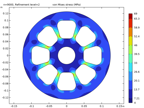
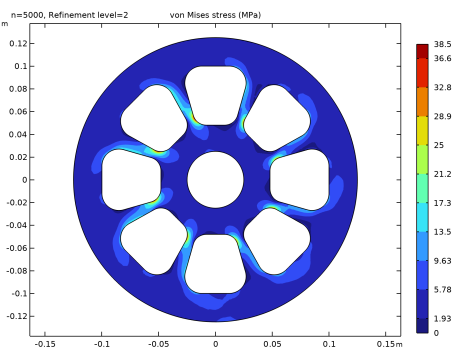
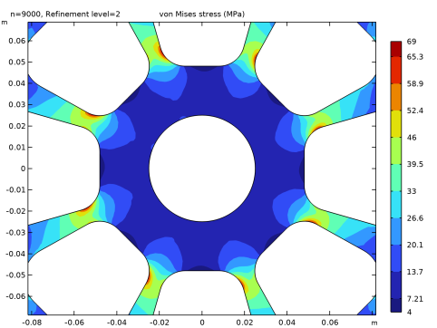
In the Settings window for Contour, click Replace Expression in the upper-right corner of the Expression section. From the menu, choose Component 1 (comp1) > Solid Mechanics > Stress > solid.misesGp - von Mises stress - N/m².
3
Locate the Expression section. From the Unit list, choose MPa.
4
Locate the Levels section. In the Total levels text field, type 10.
5
Locate the Coloring and Style section. From the Contour type list, choose Filled.
6
In the von Mises toolbar, click  Plot.
7
To visualize the results for different rotational speeds, use the solution for the desired rpm value by selecting it from the Parameter value list in the Settings window for the 2D Plot Group.
von Mises
1
In the Model Builder window, click von Mises.
2
In the Settings window for 2D Plot Group, locate the Data section.
3
From the Parameter value (n) list, choose 1000.
4
In the von Mises toolbar, click  Plot.
5
Click the  Zoom Extents button in the Graphics toolbar.
6
From the Parameter value (n) list, choose 5000.
7
In the von Mises toolbar, click  Plot.
8
From the Parameter value (n) list, choose 9000.
9
In the von Mises toolbar, click  Plot.
To get a line plot of the von Mises stress at a specific point as a function of the rotational speed, make use of the feature Cut Point 2D in a 1D Plot Group.
Cut Point 2D 1
1
In the Results toolbar, click  Cut Point 2D.
2
In the Settings window for Cut Point 2D, locate the Data section.
3
From the Dataset list, choose Study 1/Parametric Solutions 1 (sol3).
4
Locate the Point Data section. In the X text field, type 0.019.
5
In the Y text field, type 0.054.
von Mises vs. Rotational Speed
1
In the Results toolbar, click  1D Plot Group.
2
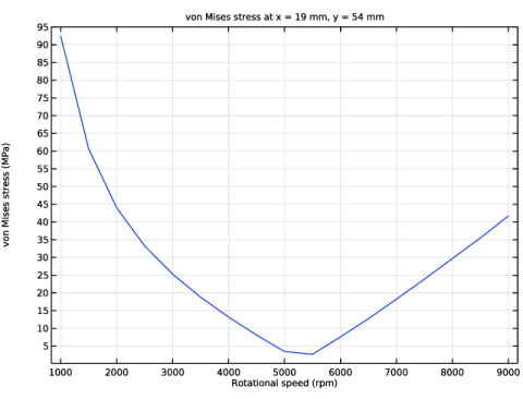
In the Settings window for 1D Plot Group, type von Mises vs. Rotational Speed in the Label text field.
3
Locate the Data section. From the Dataset list, choose Cut Point 2D 1.
4
From the Parameter selection (Refinement level) list, choose Last.
Point Graph 1
1
Right-click von Mises vs. Rotational Speed and choose Point Graph.
2
In the Settings window for Point Graph, click Replace Expression in the upper-right corner of the y-Axis Data section. From the menu, choose Component 1 (comp1) > Solid Mechanics > Stress > solid.misesGp - von Mises stress - N/m².
3
Locate the y-Axis Data section. From the Unit list, choose MPa.
4
Locate the x-Axis Data section. From the Axis source data list, choose n.
von Mises vs. Rotational Speed
1
In the Model Builder window, click von Mises vs. Rotational Speed.
2
In the Settings window for 1D Plot Group, locate the Plot Settings section.
3
Select the x-axis label checkbox. In the associated text field, type Rotational speed (rpm).
4
Click to expand the Title section. From the Title type list, choose Manual.
5
In the Title text area, type von Mises stress at x = 19 mm, y = 54 mm.
Notice that by selecting different solution-set entries in the Dataset list in the Settings window for the 1D and 2D plot groups, you can visualize results at different mesh refinements.
6
In the von Mises vs. Rotational Speed toolbar, click  Plot.
7
Click the  Zoom Extents button in the Graphics toolbar.
von Mises
Finally, zoom in on the center of the pulley to get a close-up view of the stress distribution. In particular, notice that the accurate derivative recovery method gives a smoother and more accurate solution.
1
Click the  Zoom In button in the Graphics toolbar.