PDF

Implementing a Point Source
Introduction
Consider Poisson’s equation on the unit circle with a point source at the origin. Its formal expression is:
where δ is the Dirac δ distribution located at the origin. The exact solution to this boundary value problem is −(1/2π)log(r), which has a singularity at the origin. You can model the point source by adding a Point Source node to your COMSOL Multiphysics model.
Application Library path: COMSOL_Multiphysics/Equation_Based/point_source
Modeling Instructions
From the File menu, choose New.
New
In the New window, click  Model Wizard.
Model Wizard
1
In the Model Wizard window, click  2D.
2
In the Select Physics tree, select Mathematics > Classical PDEs > Laplace’s Equation (lpeq).
3
Click Add.
4
Click  Study.
5
In the Select Study tree, select General Studies > Stationary.
6
Geometry
Circle 1 (c1)
In the Geometry toolbar, click  Circle.
Point 1 (pt1)
1
In the Geometry toolbar, click  Point.
2
In the Settings window for Point, click  Build All Objects.
Laplace’s Equation (lpeq)
Dirichlet Boundary Condition 1
1
In the Physics toolbar, click  Boundaries and choose Dirichlet Boundary Condition.
2
In the Settings window for Dirichlet Boundary Condition, locate the Boundary Selection section.
3
From the Selection list, choose All boundaries.
Point Source 1
1
In the Physics toolbar, click  Points and choose Point Source.
2
3
In the Settings window for Point Source, locate the Source Term section.
4
In the f text field, type 1.
Study 1
Step 1: Stationary
1
In the Model Builder window, under Study 1 click Step 1: Stationary.
2
In the Settings window for Stationary, click to expand the Adaptation and Error Estimates section.
3
From the Adaptation and error estimates list, choose Adaptation and error estimates.
4
In the Study toolbar, click  Compute.
Results
1
In the Settings window for 2D Plot Group, locate the Color Legend section.
2
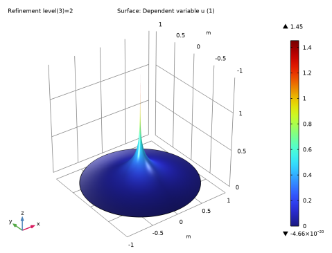
Select the Show maximum and minimum values checkbox.
Height Expression 1
1
In the Model Builder window, expand the Laplace’s Equation node.
2
Right-click Surface 1 and choose Height Expression.
The height plot appears directly.
Cut Line 2D 1
1
In the Results toolbar, click  Cut Line 2D.
2
In the Settings window for Cut Line 2D, locate the Data section.
3
From the Dataset list, choose Study 1/Adaptive Mesh Refinement Solutions 1 (sol2).
4
Locate the Line Data section. In row Point 1, set X to 0.02.
5
1D Plot Group 2
1
In the Results toolbar, click  1D Plot Group.
2
In the Settings window for 1D Plot Group, locate the Data section.
3
From the Dataset list, choose Cut Line 2D 1.
4
From the Parameter selection (Refinement level) list, choose Last.
Line Graph 1
1
Right-click 1D Plot Group 2 and choose Line Graph.
2
In the Settings window for Line Graph, locate the y-Axis Data section.
3
In the Expression text field, type u+log(x^2)/(4*pi).
4
In the 1D Plot Group 2 toolbar, click  Plot.
The resulting plot shows the error in the solution.
Surface Integration 1
1
In the Results toolbar, click  More Derived Values and choose Integration > Surface Integration.
2
In the Settings window for Surface Integration, locate the Data section.
3
From the Dataset list, choose Study 1/Adaptive Mesh Refinement Solutions 1 (sol2).
4
From the Parameter selection (Refinement level) list, choose Last.
5
6
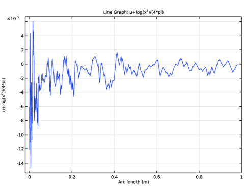
Locate the Expressions section. In the table, enter the following settings:
7
Click  Evaluate.
Table 1
1
Go to the Table 1 window.
The result of this integration shows that the error is small.