|
|
|


|
1
|
|
2
|
|
3
|
Click Add.
|
|
4
|
Click
|
|
5
|
|
6
|
Click
|
|
1
|
|
2
|
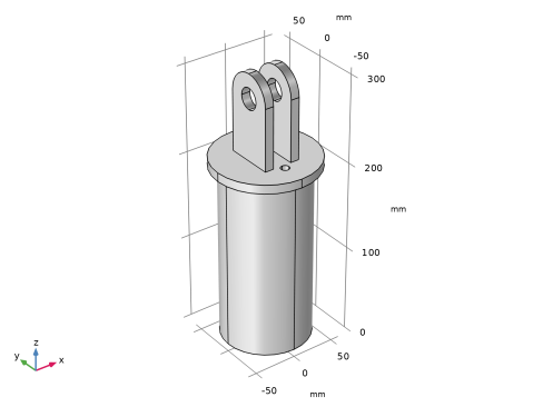
Browse to the model’s Application Libraries folder and double-click the file mast_diagonal_mounting_geom_sequence.mph.
|
|
3
|
|
4
|
|
5
|
|
1
|
|
2
|
|
1
|
|
2
|
|
3
|
|
5
|
Click
|
|
6
|
|
7
|
Click OK.
|
|
1
|
|
2
|
|
1
|
|
2
|
Go to the Add Material window.
|
|
3
|
|
4
|
Click the Add to Component button in the window toolbar.
|
|
5
|
|
1
|
|
1
|
|
3
|
|
4
|
|
1
|
|
2
|
|
3
|
|
1
|
|
2
|
|
3
|
|
1
|
|
2
|
|
3
|
|
1
|
|
2
|
|
3
|
|
1
|
|
2
|
|
4
|
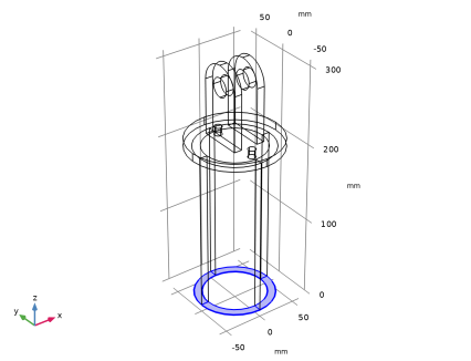
Click to expand the Destination Faces section. Select Boundary 3 only.
|
|
1
|
|
2
|
|
3
|
|
1
|
|
2
|
|
3
|
|
1
|
|
1
|
|
2
|
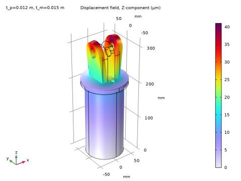
In the Settings window for Volume, click Replace Expression in the upper-right corner of the Expression section. From the menu, choose Component 1 (comp1) > Solid Mechanics > Displacement > Displacement field - m > w - Displacement field, Z-component.
|
|
3
|
|
4
|
|
5
|
|
1
|
|
2
|
In the Settings window for Global Evaluation, click Replace Expression in the upper-right corner of the Expressions section. From the menu, choose Component 1 (comp1) > Definitions > Variables > S_R - Stiffness ratio - 1.
|
|
3
|
Click
|
|
1
|
Go to the Table 1 window.
|
|
1
|
|
2
|
|
3
|
Click
|
|
5
|
Click
|
|
7
|
|
8
|
|
1
|
|
2
|
|
3
|
|
4
|
|
5
|
|
1
|
|
2
|
|
3
|
|
4
|
Click Replace Expression in the upper-right corner of the Expressions section. From the menu, choose Component 1 (comp1) > Definitions > Variables > S_R - Stiffness ratio - 1.
|
|
5
|
Click
|
|
1
|
Go to the Table 2 window.
|