|
|
|


|
1
|
|
2
|
|
3
|
Click Add.
|
|
4
|
|
5
|
Click
|
|
6
|
|
7
|
Click
|
|
1
|
In the Model Builder window, click the root node.
|
|
2
|
|
3
|
|
1
|
|
2
|
|
3
|
|
4
|
Click
|
|
1
|
|
2
|
|
3
|
|
4
|
|
5
|
|
6
|
Click
|
|
1
|
|
2
|
|
3
|
|
4
|
|
5
|
|
6
|
|
7
|
|
8
|
Click
|
|
1
|
|
2
|
Select the object elp1 only.
|
|
3
|
|
4
|
|
5
|
Select the object blk1 only.
|
|
6
|
Click
|
|
1
|
|
2
|
|
3
|
|
4
|
|
5
|
|
6
|
|
7
|
|
8
|
Click
|
|
1
|
|
2
|
Select the object sph1 only.
|
|
3
|
|
4
|
|
5
|
Select the object blk2 only.
|
|
6
|
Click
|
|
1
|
|
2
|
Click in the Graphics window and then press Ctrl+A to select both objects.
|
|
3
|
|
1
|
|
2
|
|
3
|
Select the Keep input objects checkbox.
|
|
4
|
Select the object uni1 only.
|
|
5
|
|
6
|
Click
|
|
7
|
|
1
|
|
2
|
Select the object uni1 only.
|
|
3
|
|
4
|
|
5
|
Select the object sca1 only.
|
|
6
|
Click
|
|
1
|
|
2
|
|
3
|
|
4
|
|
5
|
|
6
|
|
7
|
|
8
|
|
9
|
|
10
|
Click
|
|
1
|
|
2
|
Click in the Graphics window and then press Ctrl+A to select both objects.
|
|
3
|
|
4
|
Clear the Keep interior boundaries checkbox.
|
|
5
|
Click
|
|
1
|
|
2
|
|
1
|
In the Model Builder window, under Component 1 (comp1) > General Form PDE (g) click General Form PDE 1.
|
|
2
|
|
3
|
Specify the second Γ vector as
|
|
4
|
Locate the Source Term section. In the f text-field array, type (alpha-u1)*(u1-1)*u1-u2 on the first row.
|
|
5
|
|
1
|
|
2
|
|
3
|
|
4
|
|
1
|
|
2
|
|
3
|
|
4
|
|
1
|
|
2
|
|
3
|
|
4
|
Click
|
|
5
|
|
6
|
Click OK.
|
|
7
|
|
8
|
Click
|
|
9
|
|
1
|
|
2
|
|
3
|
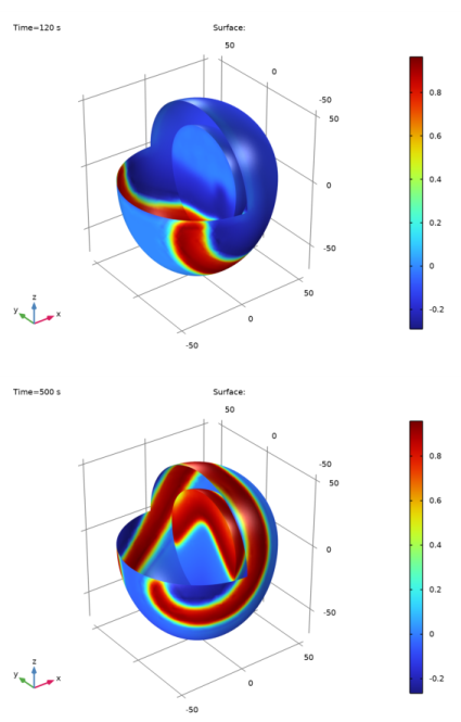
Clear the Plot dataset edges checkbox.
|
|
1
|
|
2
|
|
3
|
|
1
|
|
2
|
|
3
|
|
4
|
|
1
|
|
2
|
Go to the Add Physics window.
|
|
3
|
|
4
|
|
5
|
|
6
|
In the Dependent variables (1) table, enter the following settings:
|
|
7
|
Find the Physics interfaces in study subsection. In the table, clear the Solve checkbox for Study 1.
|
|
8
|
Click the Add to Component 1 button in the window toolbar.
|
|
9
|
|
1
|
|
2
|
Go to the Add Study window.
|
|
3
|
Find the Physics interfaces in study subsection. In the table, clear the Solve checkbox for General Form PDE (g).
|
|
4
|
|
5
|
Click the Add Study button in the window toolbar.
|
|
6
|
|
1
|
|
1
|
|
2
|
|
3
|
|
1
|
In the Model Builder window, under Component 1 (comp1) > General Form PDE 2 (g2) click General Form PDE 1.
|
|
2
|
|
3
|
Specify the first Γ vector as
|
|
4
|
Specify the second Γ vector as
|
|
5
|
Locate the Source Term section. In the f text-field array, type v1-(v1-c3*v2)*(v1^2+v2^2) on the first row.
|
|
6
|
|
1
|
|
2
|
|
3
|
|
4
|
|
1
|
|
2
|
|
3
|
|
4
|
|
5
|
|
1
|
|
2
|
|
3
|
|
4
|
|
5
|
|
6
|
|
1
|
|
2
|
|
3
|
|
4
|
|
1
|
|
2
|
|
3
|
|
4
|
|
1
|
|
2
|
In the Settings window for Surface, click Replace Expression in the upper-right corner of the Expression section. From the menu, choose Component 1 (comp1) > General Form PDE 2 > v1 - Dependent variable v1 - 1.
|
|
3
|
|
1
|
|
2
|
|
3
|
|
4
|