PDF

Deformation of a Feeder Clamp
Introduction
This example, from the field of structural mechanics, analyzes the deformation of a feeder clamp under stress. The clamp secures a feeder that carries high-frequency electromagnetic fields, and it is important that it remains as straight as possible.
This example analyzes deformations in the clamp with the following questions in mind:
Model Definition
In this analysis, the feeder clamp is bolted to a wall. The fastening can be made using either one or two mounting holes. The mounting using two holes represents a case when the fastening is properly made while fastening using only one hole represents a case when the clamp is poorly secured. The external forces on the clamp are introduced from the feeder as well as from the clamping screw, as shown in Figure 1.
.
Figure 1: Applied forces.
Loading Data
The clamp is made of aluminum. Assume that an installation technician fastens the feeder into the clamp using a standard metric M3 screw of Class 8.8 (where the first digit stands for a breaking load of 800 N/mm2, and the second digit indicates a yield strength of 80% of the breaking strength). Prestressing the screw to the yield limit results in a screw force of 4500 N. This application tests if a screw force of 20% of this value is adequate. A 7-mm washer distributes the prestressed load evenly onto both sides of the sleeve. The maximum load from the feeder onto the clamp is 2000 N, and is applied evenly throughout the inner surface of the sleeve.
Due to symmetry in both loading and the geometry, you can perform a complete model analysis while looking at only one half of the geometry. For illustrative purposes though, this example models the entire geometry.
Results and Discussion
The deformation of the loaded clamp when secured with two bolts is shown in Figure 2. In Figure 3 the deformation is shown when fastening is made using only one bolt. The results indicate clearly a larger deformation when one fastening element is missing.
Figure 2: Displacement of the clamp in the loading direction in case of two mounting bolts.
.
Figure 3: Displacement of the clamp in the loading direction in case of only one mounting bolt.
Since the problem is symmetric in the yz-plane the minimum separation of 0.5 mm can be visualized by evaluation of the expression abs(u)  >  0.25 mm, shown in Figure 4. The domains that are not colored green experience a greater displacement than 0.25 mm. Due to symmetry, this corresponds to the part of the clamp that undergoes a larger deformation than 0.5 mm, which is the minimum requirement for being able to fasten the feeder adequately. The boundary conditions in this example are valid only as long as the installation technician does not squeeze the gap in the clamping sleeve completely shut. However, if the gap is squeezed shut, you can be sure that the requirements are fulfilled.
Figure 4: Clamp deformation caused by the screw force.
The rotation of the clamp is evaluated using the rotation tensor. Since deformations are small, the components of the rotation tensor equal the angle given in radians. In Figure 5, the results are displayed in degrees. The rotation varies slightly over the generatrix of the inner sleeve surface. The computation gives an inclination value of approximately 0.5 degrees when both mounting bolts are present and tightened properly. This value is less than the maximum allowed angle of 1 degree. However, if one of the bolts is missing, the angle increases to approximately 1.75 degrees, which significantly exceeds the allowed inclination.
Figure 5: Rotation along the clamp.
Application Library path: COMSOL_Multiphysics/Structural_Mechanics/feeder_clamp
Modeling Instructions
From the File menu, choose New.
New
In the New window, click  Model Wizard.
Model Wizard
1
In the Model Wizard window, click  3D.
2
In the Select Physics tree, select Structural Mechanics > Solid Mechanics (solid).
3
Click Add.
4
Click  Study.
5
In the Select Study tree, select General Studies > Stationary.
6
Global Definitions
Parameters 1
1
In the Model Builder window, under Global Definitions click Parameters 1.
2
In the Settings window for Parameters, locate the Parameters section.
3
To add a parameter, you can either edit directly in an empty table row or use the text fields below the table and click Move Up when you are finished (you might need to click on the table row to activate the text fields first).
Geometry 1
1
In the Model Builder window, under Component 1 (comp1) click Geometry 1.
2
In the Settings window for Geometry, locate the Units section.
3
From the Length unit list, choose mm.
Block 1 (blk1)
1
In the Geometry toolbar, click  Block.
2
In the Settings window for Block, locate the Size and Shape section.
3
In the Width text field, type 30[mm].
4
In the Depth text field, type 40[mm].
5
In the Height text field, type 5[mm].
6
Locate the Position section. In the y text field, type -30[mm].
Work Plane 1 (wp1)
1
In the Geometry toolbar, click  Work Plane.
2
In the Settings window for Work Plane, locate the Plane Definition section.
3
From the Plane list, choose yz-plane.
4
In the x-coordinate text field, type 5[mm].
Work Plane 1 (wp1) > Plane Geometry
In the Model Builder window, click Plane Geometry.
Work Plane 1 (wp1) > Rectangle 1 (r1)
1
In the Work Plane toolbar, click  Rectangle.
2
In the Settings window for Rectangle, locate the Size and Shape section.
3
In the Width text field, type 10[mm].
4
In the Height text field, type 55[mm].
5
Locate the Position section. In the xw text field, type -15[mm].
6
In the yw text field, type 5[mm].
Work Plane 1 (wp1) > Fillet 1 (fil1)
1
In the Work Plane toolbar, click  Fillet.
2
On the object r1, select Points 3 and 4 only.
3
In the Settings window for Fillet, locate the Radius section.
4
In the Radius text field, type 5[mm].
Work Plane 1 (wp1) > Circle 1 (c1)
1
In the Work Plane toolbar, click  Circle.
2
In the Settings window for Circle, locate the Size and Shape section.
3
In the Radius text field, type 3.5[mm].
4
Locate the Position section. In the xw text field, type -10[mm].
5
In the yw text field, type 55[mm].
Work Plane 1 (wp1) > Circle 2 (c2)
1
Right-click Component 1 (comp1) > Geometry 1 > Work Plane 1 (wp1) > Plane Geometry > Circle 1 (c1) and choose Duplicate.
2
In the Settings window for Circle, locate the Size and Shape section.
3
In the Radius text field, type 1.875[mm].
Work Plane 1 (wp1) > Difference 1 (dif1)
1
In the Work Plane toolbar, click  Booleans and Partitions and choose Difference.
2
Select the objects c1 and fil1 only.
3
In the Settings window for Difference, locate the Difference section.
4
Click to select the  Activate Selection toggle button for Objects to subtract.
5
6
Click  Build Selected.
Extrude 1 (ext1)
1
In the Model Builder window, under Component 1 (comp1) > Geometry 1 right-click Work Plane 1 (wp1) and choose Extrude.
2
In the Settings window for Extrude, locate the Distances section.
3
4
Click  Build Selected.
Cylinder 1 (cyl1)
1
In the Geometry toolbar, click  Cylinder.
2
In the Settings window for Cylinder, locate the Size and Shape section.
3
In the Radius text field, type 15[mm].
4
In the Height text field, type 20[mm].
5
Locate the Position section. In the x text field, type 15[mm].
6
In the y text field, type -20[mm].
7
In the z text field, type 35[mm].
8
Locate the Axis section. From the Axis type list, choose y-axis.
Union 1 (uni1)
1
In the Geometry toolbar, click  Booleans and Partitions and choose Union.
2
Select the objects cyl1 and ext1 only.
3
In the Settings window for Union, locate the Union section.
4
Clear the Keep interior boundaries checkbox.
Partition the geometry to enable structured meshing.
Partition Faces 1 (parf1)
1
In the Geometry toolbar, click  Booleans and Partitions and choose Partition Faces.
2
On the object uni1, select Boundaries 1, 2, 19, and 20 only.
3
In the Settings window for Partition Faces, locate the Partition Faces section.
4
From the Partition with list, choose Extended edges.
5
On the object uni1, select Edges 9, 12, 50, and 52 only.
Partition Domains 1 (pard1)
1
In the Geometry toolbar, click  Booleans and Partitions and choose Partition Domains.
2
On the object parf1, select Domain 1 only.
3
In the Settings window for Partition Domains, locate the Partition Domains section.
4
From the Partition with list, choose Extended faces.
5
On the object parf1, select Boundary 2 only.
Cylinder 2 (cyl2)
1
In the Geometry toolbar, click  Cylinder.
2
In the Settings window for Cylinder, locate the Size and Shape section.
3
In the Radius text field, type 10[mm].
4
In the Height text field, type 20[mm].
5
Locate the Position section. In the x text field, type 15[mm].
6
In the y text field, type -20[mm].
7
In the z text field, type 35[mm].
8
Locate the Axis section. From the Axis type list, choose y-axis.
Block 2 (blk2)
1
In the Geometry toolbar, click  Block.
2
In the Settings window for Block, locate the Size and Shape section.
3
In the Width text field, type 1.5[mm].
4
In the Depth text field, type 20[mm].
5
In the Height text field, type 20[mm].
6
Locate the Position section. In the x text field, type 14.25[mm].
7
In the y text field, type -20[mm].
8
In the z text field, type 40[mm].
Work Plane 2 (wp2)
1
In the Geometry toolbar, click  Work Plane.
2
In the Settings window for Work Plane, locate the Plane Definition section.
3
From the Plane type list, choose Face parallel.
4
On the object blk1, select Boundary 1 only.
Work Plane 2 (wp2) > Plane Geometry
In the Model Builder window, click Plane Geometry.
Work Plane 2 (wp2) > Rectangle 1 (r1)
1
In the Work Plane toolbar, click  Rectangle.
2
In the Settings window for Rectangle, locate the Size and Shape section.
3
In the Width text field, type 11[mm].
4
In the Height text field, type 5[mm].
5
Locate the Position section. In the xw text field, type -5.5[mm].
6
In the yw text field, type -15[mm].
Work Plane 2 (wp2) > Circle 1 (c1)
1
In the Work Plane toolbar, click  Circle.
2
In the Settings window for Circle, locate the Size and Shape section.
3
In the Radius text field, type 2.5[mm].
4
Locate the Position section. In the xw text field, type -5.5[mm].
5
In the yw text field, type -12.5[mm].
Work Plane 2 (wp2) > Circle 2 (c2)
1
Right-click Component 1 (comp1) > Geometry 1 > Work Plane 2 (wp2) > Plane Geometry > Circle 1 (c1) and choose Duplicate.
2
In the Settings window for Circle, locate the Position section.
3
In the xw text field, type 5.5[mm].
Work Plane 2 (wp2) > Mirror 1 (mir1)
1
In the Work Plane toolbar, click  Transforms and choose Mirror.
2
Click in the Graphics window and then press Ctrl+A to select all objects.
3
In the Settings window for Mirror, locate the Normal Vector to Line of Reflection section.
4
In the xw text field, type 0.
5
In the yw text field, type 1.
6
Locate the Input section. Select the Keep input objects checkbox.
7
Click  Build Selected.
Extrude 2 (ext2)
1
In the Model Builder window, under Component 1 (comp1) > Geometry 1 right-click Work Plane 2 (wp2) and choose Extrude.
2
In the Settings window for Extrude, locate the Distances section.
3
From the Specify list, choose Vertices to extrude to.
4
On the object blk1, select Point 7 only.
Difference 1 (dif1)
1
In the Geometry toolbar, click  Booleans and Partitions and choose Difference.
2
Select the objects blk1 and pard1 only.
3
In the Settings window for Difference, locate the Difference section.
4
Click to select the  Activate Selection toggle button for Objects to subtract.
5
Select the objects blk2, cyl2, and ext2 only.
Partition Faces 2 (parf2)
1
In the Geometry toolbar, click  Booleans and Partitions and choose Partition Faces.
2
On the object dif1, select Boundary 17 only.
3
In the Settings window for Partition Faces, locate the Partition Faces section.
4
Click to select the  Activate Selection toggle button for Vertices defining curve segments.
5
On the object dif1, select Points 57 and 58 only.
Form Union (fin)
1
In the Model Builder window, click Form Union (fin).
2
In the Settings window for Form Union/Assembly, click  Build Selected.
3
Click  Build Selected.
4
Click the  Go to Default View button in the Graphics toolbar.
Add Material
1
In the Materials toolbar, click  Add Material to open the Add Material window.
2
Go to the Add Material window.
3
In the tree, select Built-in > Aluminum.
4
Click the Add to Component button in the window toolbar.
5
In the Materials toolbar, click  Add Material to close the Add Material window.
Solid Mechanics (solid)
The boundary conditions consist of loads and constraints. The latter model the mounting bolts by setting the displacement to zero at the mounting holes off the clamp. All other boundaries are free.
Boundary Load 1
1
In the Physics toolbar, click  Boundaries and choose Boundary Load.
2
It might be easier to select the correct boundary by using the Selection List window. To open this window, in the Home toolbar click Windows and choose Selection List. (If you are running the cross-platform desktop, you find Windows in the main menu.)
3
In the Settings window for Boundary Load, locate the Force section.
4
From the Load type list, choose Total force.
5
Specify the Ftot vector as
Boundary Load 2
1
In the Physics toolbar, click  Boundaries and choose Boundary Load.
2
3
In the Settings window for Boundary Load, locate the Force section.
4
From the Load type list, choose Total force.
5
Specify the Ftot vector as
Boundary Load 3
1
In the Physics toolbar, click  Boundaries and choose Boundary Load.
2
3
In the Settings window for Boundary Load, locate the Force section.
4
From the Load type list, choose Total force.
5
Specify the Ftot vector as
Fixed Constraint 1
1
In the Physics toolbar, click  Boundaries and choose Fixed Constraint.
2
Assign the constraint grouping to be able to disable or enable the corresponding constraint in a parametric analysis.
3
In the Physics toolbar, click  Constraint Group and choose New Constraint Group.
Fixed Constraint 2
1
Right-click Fixed Constraint 1 and choose Duplicate.
2
3
In the Physics toolbar, click  Constraint Group and choose New Constraint Group.
Mesh 1
Swept 1
In the Mesh toolbar, click  Swept.
Size
1
In the Model Builder window, click Size.
2
In the Settings window for Size, locate the Element Size section.
3
From the Predefined list, choose Extremely fine.
Swept 1
1
In the Model Builder window, click Swept 1.
2
In the Settings window for Swept, click to expand the Source Faces section.
3
4
Click  Build All.
Study 1
Step 1: Stationary
1
In the Model Builder window, under Study 1 click Step 1: Stationary.
2
In the Settings window for Stationary, click to expand the Study Extensions section.
Set up two load cases: the first one with both mounting bolts present and the second one with one of the bolts either loose or missing completely.
3
Select the Define load cases checkbox.
4
5
6
Solution 1 (sol1)
1
In the Study toolbar, click  Show Default Solver.
2
In the Model Builder window, expand the Solution 1 (sol1) node, then click Stationary Solver 1.
3
In the Settings window for Stationary Solver, click to expand the Output section.
4
Clear the Reaction forces checkbox.
5
In the Study toolbar, click  Compute.
Results
The default plot shows the stress distribution over the deformed geometry. Change it to visualize the displacement in the loading direction.
y-Displacement LC1
1
In the Model Builder window, under Results click Stress (solid).
2
In the Settings window for 3D Plot Group, type y-Displacement LC1 in the Label text field.
3
Locate the Color Legend section. Select the Show units checkbox.
Volume 1
1
In the Model Builder window, expand the y-Displacement LC1 node, then click Volume 1.
2
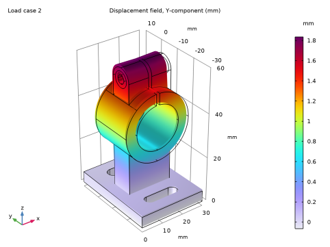
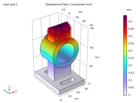
In the Settings window for Volume, click Replace Expression in the upper-right corner of the Expression section. From the menu, choose Component 1 (comp1) > Solid Mechanics > Displacement > Displacement field - m > v - Displacement field, Y-component.
3
In the y-Displacement LC1 toolbar, click  Plot.
4
Click the  Zoom Extents button in the Graphics toolbar.
The plot seems to indicate that the gap in the sleeve has been shut. However, this is an artifact of the default scale factor being larger than 1. To get an accurate view of the size of the deformation, set the scale factor to 1.
Deformation
1
In the Model Builder window, expand the Volume 1 node, then click Deformation.
2
In the Settings window for Deformation, locate the Scale section.
3
Select the Scale factor checkbox. In the associated text field, type 1.
y-Displacement LC1
1
In the Model Builder window, under Results click y-Displacement LC1.
2
In the Settings window for 3D Plot Group, locate the Data section.
3
From the Load case list, choose Load case 1.
4
In the y-Displacement LC1 toolbar, click  Plot.
5
Click the  Zoom Extents button in the Graphics toolbar.
The resulting plot should be similar to that shown in Figure 2. Thus, there is still a narrow gap in the sleeve (if necessary, rotate the geometry in the Graphics window to get a better view).
y-Displacement LC2
Now, duplicate the plot to shown the second case with one of the mounting bolts missing, Figure 3.
1
Right-click y-Displacement LC1 and choose Duplicate.
2
In the Settings window for 3D Plot Group, type y-Displacement LC2 in the Label text field.
3
Locate the Data section. From the Load case list, choose Load case 2.
4
In the y-Displacement LC2 toolbar, click  Plot.
5
Click the  Zoom Extents button in the Graphics toolbar.
Proceed to reproduce the plot shown in Figure 4.
x-Displacement
1
In the Results toolbar, click  3D Plot Group.
2
In the Settings window for 3D Plot Group, type x-Displacement in the Label text field.
3
Locate the Color Legend section. Select the Show units checkbox.
Surface 1
1
Right-click x-Displacement and choose Surface.
2
In the Settings window for Surface, locate the Expression section.
3
In the Expression text field, type u*(abs(u)>0.25[mm]).
4
Locate the Coloring and Style section. From the Color table list, choose RainbowLight.
5
In the x-Displacement toolbar, click  Plot.
6
Click the  Zoom Extents button in the Graphics toolbar.
You can flip the Load case selector on the plot Data tab to see that the increase in inclination has almost no effect on the clamp deformation due to the screw forces.
Examine the resulting rotation of the clamp by evaluating the rotation of the deformation tensor.
Rotation
1
In the Results toolbar, click  1D Plot Group.
2
In the Settings window for 1D Plot Group, type Rotation in the Label text field.
3
Locate the Legend section. From the Position list, choose Upper left.
Line Graph 1
1
Right-click Rotation and choose Line Graph.
2
3
In the Settings window for Line Graph, click Replace Expression in the upper-right corner of the y-Axis Data section. From the menu, choose Component 1 (comp1) > Solid Mechanics > Strain > Rotation of deformation tensor > solid.RotyZ - Rotation of deformation tensor, yZ component.
4
Locate the y-Axis Data section. In the Expression text field, type solid.RotyZ*180/pi.
5
Locate the x-Axis Data section. From the Parameter list, choose Expression.
6
In the Expression text field, type Y.
7
Click to expand the Legends section. Select the Show legends checkbox.
Rotation
1
In the Model Builder window, click Rotation.
2
In the Settings window for 1D Plot Group, locate the Plot Settings section.
3
Select the y-axis label checkbox. In the associated text field, type Rotation of deformation tensor, yz-component (deg).