

PDF

Chemical Etching
Introduction
This example illustrates the principle of wet chemical etching. Wet chemical etching is particularly important for microelectronics industry for patterning of integrated circuits, MEMS devices, and optoelectronic and pressure sensors. Wet etching processes use solution based (“wet”) etchants, where the substrate to be etched is immersed in a controlled flow of etchant. Wet etching process is selective isotropic, fast (usually reaction rate limited) and reproducible. Due to its reproducibility the technique is often used for micropatterning of substrates.
A wet etching process involves chemical reaction that consume the original reactant and produce new reactant. The wet etch process can be described by three basic steps:
The purpose of this tutorial is to examine how the copper substrate material is depleted and how the cavity shape evolves during the wet etching process. The rate of the etching reaction depends on the local concentration of a reactant, which is transported to the surface by coupled convection–diffusion. The laminar flow profile of the etchant fluid changes due to the shape evolution of the etched cavity.
Model Definition
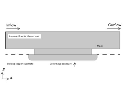
The simplified 2D model geometry consists of a masked copper substrate with an exposed surface which is to be wet etched. The geometry is shown in Figure 1. The top rectangular domain has fluid flowing over the exposed copper substrate as marked in the x direction. The fluid reacts only with the unmasked copper as the etching proceeds.
Figure 1: Schematic diagram of the chemical etching under a laminar flow of the etchant.
Transport of Chemical Species
The mass flux of the etching species is governed by diffusion and convection according to
(1)
where D (SI unit: m2/s) denotes the diffusion coefficient and (SI unit: mol/m3) is the concentration. The modeled species has a diffusion coefficient of 1 · 109 m2/s. At the inlet and top boundaries of the flow, the concentration is equal to the bulk concentration of the etchant solution. At the etching surface (moving boundary), the flux condition is considered as in:
(2)
where k (SI unit: m/s) is the forward rate constant for linear kinetics of the etching species, and n is the normal vector. k is assumed to be independent of the position on the surface. A No Flux condition is used for all other boundaries except the moving boundary.
Laminar Flow
At the cavity, the flow field can be calculated by the Navier–Stokes equations
(3)
along with the continuity equation
(4)
Here ρ is the fluid density (SI unit: kg/m3), p is the pressure (SI unit: Pa), μ is the dynamic viscosity (SI unit: Pa·s), F is the volume force vector (indicated as the boundary stress in the modeling instructions), and u is the fluid velocity (SI unit: m/s).
Along the moving wall, a no slip condition is applied.
Deformed Geometry
The movement of the boundary is defined by an interfacial condition on the boundary
(5)
where v is velocity of the moving mesh in the normal direction; r, M, and ρ are the reaction rate (SI unit: mol/(m2 ·s), which is the right side k c in Equation 2 above, molar mass (SI unit: kg/mol), and density (SI unit: kg/m3) of the etching species, respectively.
Results and Discussion
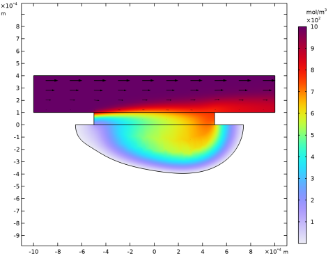
Figure 2 shows the concentration of etchant species CuCl2 at t = 10,800 s for an initial cavity radius of 0.5 mm. The etch profile is asymmetric owing to the fluid flow in the x direction. The etch rate is higher around the area where laminar flow first encounters the boundary layer in fluid direction. Concentration becomes uniform deeper into the cavity as laminar flow can no longer transport reactant to the boundary layer owing to larger aspect ratio. (See also the velocity profile in Figure 3.)
Figure 2: Concentration profile of CuCl2 etchant at t = 10,800 s over unmasked copper cavity.
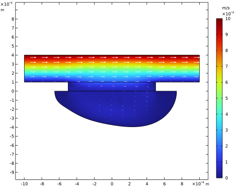
Figure 3 shows the velocity profile for etchant flow at t = 10,800 s. The velocity is zero close to the moving boundary. The fluid flow eventually becomes weak deeper as the aspect ratio of cavity increases with time.
Figure 3: Arrow surface plot depicting velocity profile of CuCl2 etchant after t = 10,800 s over the deformed geometry of copper cavity.
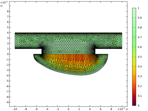
Figure 4: Mesh deformation after t = 10,800 s over the etching unmasked copper cavity.
Figure 4 shows mesh deformation for the deforming geometry at t = 10,800 s.
Reference
1. D.J. Economou and others, “Effect of Transport and Reaction on the Shape Evolution of Cavities During Wet Chemical Etching,” J. Electrochem. Soc., vol. 136, no. 7, pp. 1997–2004, 1989.
Application Library path: COMSOL_Multiphysics/Chemical_Engineering/chemical_etching
Modeling Instructions
From the File menu, choose New.
New
In the New window, click  Model Wizard.
Model Wizard
1
In the Model Wizard window, click  2D.
Add the required physics.
2
In the Select Physics tree, select Chemical Species Transport > Transport of Diluted Species (tds).
3
Click Add.
4
In the Concentration (mol/m³) text field, type cCuCl2.
5
In the Select Physics tree, select Fluid Flow > Single-Phase Flow > Laminar Flow (spf).
6
Click Add.
7
Click  Study.
8
In the Select Study tree, select General Studies > Stationary.
9
Global Definitions
Parameters 1
1
In the Model Builder window, expand the Component 1 (comp1) > Definitions node, then click Global Definitions > Parameters 1.
2
In the Settings window for Parameters, locate the Parameters section.
3
Click  Load from File.
4
Next, define the variable v_surface corresponding to the velocity of the moving boundary.
Definitions
Variables 1
1
In the Model Builder window, under Component 1 (comp1) right-click Definitions and choose Variables.
2
In the Settings window for Variables, locate the Variables section.
3
Geometry 1
Rectangle 1 (r1)
1
In the Model Builder window, expand the Component 1 (comp1) > Geometry 1 node.
2
Right-click Geometry 1 and choose Rectangle.
3
In the Settings window for Rectangle, locate the Size and Shape section.
4
In the Width text field, type d_mask.
5
In the Height text field, type h_mask.
6
Locate the Position section. In the x text field, type -0.5*d_mask.
Rectangle 2 (r2)
1
In the Geometry toolbar, click  Rectangle.
2
In the Settings window for Rectangle, locate the Size and Shape section.
3
In the Width text field, type h_boundary_layer.
4
In the Height text field, type h_seed_cavity.
5
Locate the Position section. In the x text field, type -0.5*h_boundary_layer.
6
In the y text field, type -h_seed_cavity.
Fillet 1 (fil1)
1
In the Geometry toolbar, click  Fillet.
2
Click the  Zoom Extents button in the Graphics toolbar.
3
On the object r2, select Points 1 and 2 only.
4
In the Settings window for Fillet, locate the Radius section.
5
In the Radius text field, type h_seed_cavity/2.
Rectangle 3 (r3)
1
In the Geometry toolbar, click  Rectangle.
2
In the Settings window for Rectangle, locate the Size and Shape section.
3
In the Width text field, type d_mask*2.
4
In the Height text field, type 3*h_mask.
5
Locate the Position section. In the x text field, type -d_mask.
6
In the y text field, type h_mask.
7
Click  Build All Objects.
Definitions
Moving Boundary
1
In the Definitions toolbar, click  Box.
2
In the Settings window for Box, locate the Geometric Entity Level section.
3
From the Level list, choose Boundary.
4
In the Label text field, type Moving Boundary.
5
Locate the Box Limits section. In the y maximum text field, type -h_seed_cavity*0.001.
Bottom
1
Right-click Moving Boundary and choose Duplicate.
2
In the Settings window for Box, type Bottom in the Label text field.
3
Locate the Box Limits section. In the y maximum text field, type -h_seed_cavity*0.999.
4
Locate the Output Entities section. From the Include entity if list, choose Entity inside box.
Add Material
1
In the Materials toolbar, click  Add Material to open the Add Material window.
2
Go to the Add Material window.
3
In the tree, select Built-in > Water, liquid.
4
Click the Add to Component button in the window toolbar.
5
In the Materials toolbar, click  Add Material to close the Add Material window.
Transport of Diluted Species (tds)
Fluid 1
1
In the Model Builder window, expand the Component 1 (comp1) > Transport of Diluted Species (tds) > Fluid 1 node, then click Fluid 1.
2
In the Settings window for Fluid, locate the Convection section.
3
From the u list, choose Velocity field (spf).
4
Locate the Diffusion section. In the DcCuCl2 text field, type D.
Concentration 1
1
In the Model Builder window, expand the Component 1 (comp1) > Transport of Diluted Species (tds) > No Flux 1 node.
2
Right-click Transport of Diluted Species (tds) and choose Concentration.
3
4
In the Settings window for Concentration, locate the Concentration section.
5
Select the Species cCuCl2 checkbox.
6
In the c0,cCuCl2 text field, type cCuCl2_bulk.
Outflow 1
1
In the Physics toolbar, click  Boundaries and choose Outflow.
2
Flux 1
1
In the Physics toolbar, click  Boundaries and choose Flux.
2
In the Settings window for Flux, locate the Boundary Selection section.
3
From the Selection list, choose Moving Boundary.
4
Locate the Inward Flux section. Select the Species cCuCl2 checkbox.
5
In the J0,cCuCl2 text field, type r_surface.
Laminar Flow (spf)
In the Model Builder window, under Component 1 (comp1) click Laminar Flow (spf).
Wall 2
1
In the Physics toolbar, click  Boundaries and choose Wall.
2
3
In the Settings window for Wall, click to expand the Wall Movement section.
4
From the Translational velocity list, choose Manual.
5
Specify the utr vector as
Boundary Stress 1
1
In the Physics toolbar, click  Boundaries and choose Boundary Stress.
2
3
In the Settings window for Boundary Stress, locate the Boundary Condition section.
4
From the Boundary condition list, choose Normal stress, normal flow.
Component 1 (comp1)
Deforming Domain 1
1
In the Physics toolbar, click  Deformed Geometry and choose Free Deformation.
2
3
In the Settings window for Deforming Domain, locate the Smoothing section.
4
From the Mesh smoothing type list, choose Hyperelastic.
Prescribed Normal Mesh Velocity 1
1
In the Deformed Geometry toolbar, click  Prescribed Normal Mesh Velocity.
2
In the Settings window for Prescribed Normal Mesh Velocity, locate the Boundary Selection section.
3
From the Selection list, choose Moving Boundary.
4
Locate the Prescribed Normal Mesh Velocity section. In the vn text field, type v_surface.
Prescribed Normal Mesh Displacement 1
1
In the Deformed Geometry toolbar, click  Prescribed Normal Mesh Displacement.
2
Prescribed Mesh Displacement 1
1
In the Deformed Geometry toolbar, click  Prescribed Mesh Displacement.
2
Study 1
Step 1: Stationary
1
In the Model Builder window, under Study 1 click Step 1: Stationary.
2
In the Settings window for Stationary, locate the Physics and Variables Selection section.
3
In the Solve for column of the table, under Component 1 (comp1), clear the checkbox for Deformed Geometry.
Step 2: Time Dependent
1
In the Study toolbar, click  Time Dependent.
2
In the Settings window for Time Dependent, locate the Study Settings section.
3
In the Output times text field, type range(0,0.05*tmax,tmax).
4
In the Study toolbar, click  Compute.
Results
Concentration (tds)
1
In the Settings window for 2D Plot Group, locate the Color Legend section.
2
Select the Show units checkbox.
3
Click the  Zoom Extents button in the Graphics toolbar.
4
In the Concentration (tds) toolbar, click  Plot.
Velocity (spf)
1
In the Model Builder window, click Velocity (spf).
2
In the Settings window for 2D Plot Group, locate the Color Legend section.
3
Select the Show units checkbox.
Arrow Surface 1
1
Right-click Velocity (spf) and choose Arrow Surface.
2
In the Settings window for Arrow Surface, locate the Coloring and Style section.
3
From the Arrow length list, choose Logarithmic.
4
From the Color list, choose White.
5
In the Velocity (spf) toolbar, click  Plot.
Pressure (spf)
1
In the Model Builder window, under Results click Pressure (spf).
2
In the Settings window for 2D Plot Group, locate the Color Legend section.
3
Select the Show units checkbox.
4
Click the  Zoom Extents button in the Graphics toolbar.
5
In the Pressure (spf) toolbar, click  Plot.
Mesh
1
In the Results toolbar, click  2D Plot Group.
2
Right-click 2D Plot Group 5 and choose Rename.
3
In the Rename 2D Plot Group dialog, type Mesh in the New label text field.
4
5
In the Settings window for 2D Plot Group, type Mesh in the Label text field.
Mesh 1
1
Right-click Mesh and choose Mesh.
2
In the Mesh toolbar, click  Plot.
Animation 1
1
In the Results toolbar, click  Animation and choose Player.
2
In the Settings window for Animation, click  Show Frame.
3
Locate the Frames section. From the Frame selection list, choose All.
4
In the Frame number text field, type 101.
5
Click the  Play button in the Graphics toolbar.