
|
|
|


|
3.33·10-2
|
1.68·10-2
|
||
|
1
|
|
2
|
|
3
|
Click Add.
|
|
4
|
|
5
|
Click
|
|
6
|
In the Dependent variables (1) table, enter the following settings:
|
|
7
|
Click
|
|
8
|
|
9
|
Click
|
|
1
|
|
2
|
|
1
|
|
2
|
|
1
|
In the Model Builder window, under Component 1 (comp1) > Coefficient Form PDE (c) click Coefficient Form PDE 1.
|
|
2
|
|
3
|
|
4
|
|
5
|
Locate the Absorption Coefficient section. In the a text-field array, type 1 in the second column of the first row.
|
|
6
|
|
7
|
|
8
|
Locate the Damping or Mass Coefficient section. In the da text-field array, type 0 in the first column of the first row.
|
|
9
|
|
10
|
Click to expand the Convection Coefficient section. In the β text-field array, type -1 in the first column of the first row.
|
|
11
|
|
1
|
|
1
|
|
2
|
|
4
|
In the Settings window for Dirichlet Boundary Condition, locate the Dirichlet Boundary Condition section.
|
|
5
|
Clear the Prescribed value of f checkbox.
|
|
6
|
|
1
|
|
2
|
|
3
|
|
1
|
|
2
|
|
3
|
|
4
|
|
5
|
|
6
|
|
7
|
Click
|
|
1
|
|
2
|
|
3
|
|
4
|
|
1
|
|
2
|
In the Model Builder window, expand the Study 1 > Solver Configurations > Solution 1 (sol1) > Stationary Solver 1 node, then click Direct.
|
|
3
|
|
4
|
|
5
|
|
6
|
|
7
|
|
8
|
Click OK.
|
|
1
|
|
2
|
|
3
|
|
4
|
|
5
|
|
1
|
|
2
|
|
3
|
|
4
|
Locate the Plot Settings section.
|
|
5
|
|
6
|
|
7
|
|
8
|
|
9
|
|
10
|
|
11
|
|
12
|
|
13
|
|
1
|
|
2
|
|
4
|
|
5
|
|
1
|
|
2
|
Go to the Add Physics window.
|
|
3
|
|
4
|
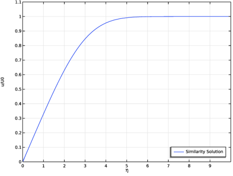
Find the Physics interfaces in study subsection. In the table, clear the Solve checkbox for Similarity Solution.
|
|
5
|
Click the Add to Component 2 button in the window toolbar.
|
|
6
|
|
1
|
|
2
|
Go to the Add Study window.
|
|
3
|
|
4
|
Click the Add Study button in the window toolbar.
|
|
5
|
|
1
|
|
2
|
|
3
|
|
4
|
|
5
|
|
6
|
|
1
|
|
2
|
Click
|
|
1
|
|
2
|
|
3
|
|
4
|
|
1
|
|
2
|
Go to the Add Material window.
|
|
3
|
|
4
|
Click the Add to Component button in the window toolbar.
|
|
5
|
|
1
|
|
3
|
|
4
|
|
1
|
|
1
|
|
1
|
|
1
|
|
3
|
|
4
|
|
1
|
|
3
|
|
4
|
|
1
|
|
3
|
|
4
|
|
5
|
|
6
|
|
7
|
|
8
|
Click
|
|
1
|
|
2
|
|
3
|
Click
|
|
1
|
|
2
|
|
3
|
Find the Values of variables not solved for subsection. From the Settings list, choose User controlled.
|
|
4
|
|
5
|
|
6
|
|
7
|
|
1
|
|
2
|
|
3
|
In the Model Builder window, expand the Study 2 > Solver Configurations > Solution 2 (sol2) > Stationary Solver 1 node, then click Fully Coupled 1.
|
|
4
|
|
5
|
|
6
|
|
1
|
|
2
|
|
3
|
|
4
|
|
5
|
|
1
|
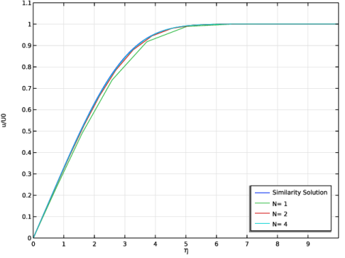
In the Model Builder window, under Results > Coefficient Form PDE right-click Line Graph 1 and choose Duplicate.
|
|
2
|
|
3
|
|
4
|
|
5
|
|
6
|
|
7
|
|
8
|
|
1
|
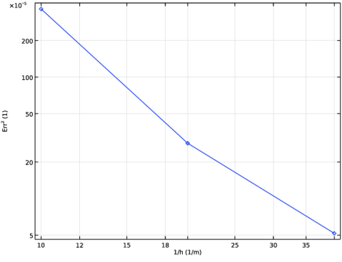
In the Model Builder window, under Results right-click Derived Values and choose Integration > Line Integration.
|
|
2
|
|
3
|
|
4
|
|
6
|
Click
|
|
1
|
|
3
|
|
5
|
|
6
|
Click the arrow next to the Evaluate button and choose Table 1 - Line Integration 1 ((u/U0-comp1.genext1(fprime))^2/sqrt(b0*x)).
|
|
1
|
Go to the Table 1 window.
|
|
2
|
Click the Table Graph button in the window toolbar.
|
|
1
|
|
2
|
|
3
|
|
4
|
|
5
|
Locate the Coloring and Style section. Find the Line markers subsection. From the Marker list, choose Diamond.
|
|
6
|
|
7
|