COMSOL 6.4 - The Black–Scholes Equation

PDF

The Black–Scholes Equation

There are different types of stock options:

•

A call option is the right to buy a security at a specified price (called the exercise or strike price) during a specified period of time.

•

A put option is the right to sell a security at a specified price during a specified period of time.

American options can be exercised at any time up to and including the day the option expires. European options can be exercised only on the day the option expires.

The famous Black–Scholes equation computes the cost u of a European stock option

with the following parameters:

•

x, the underlying asset price

•

r, the continuous compounding rate of interest

•

σ, the standard deviation of the asset’s rate of return (also known as volatility)

A put option’s value on the exercise day is

where K is the strike price. The problem domain is infinite and consists of the entire real axis across the time domain 0 ≤ t ≤ T.

The assumptions made in deriving the Black-Scholes equation are:

•

The underlying stock pays no dividends.

•

The price of the stock, one period ahead, has a log-normal distribution with mean and standard deviation that are constant over the life of the option.

•

The existence of a risk-free interest rate which is constant over the life of the option.

•

You can lend and borrow at the risk-free interest rate.

Black and Scholes derived an analytical expression for the solution to the above problem. However, the formula works only for certain cases. For instance, you cannot use it when σ and r are functions of x and t. Using the PDE formulation, you can determine the price for such cases.

Model Definition

Because you work within a finite domain 0 ≤ x ≤ X, it is necessary to specify not only the boundary conditions for t = T but also for x = 0 and x = X. It is therefore necessary to analyze the problem’s characteristics to determine the location of the input and output boundaries.

Equation Definition

To put the equation in coefficient form, rewrite the equation as

In the following, denote

To reduce the problems with inflow boundaries, start by considering a put option: Study the value of a put option at a strike price K = 40 with σ = 0.3 and r = 0.12.

Boundary Conditions and Initial Conditions

Make the domain be 0 ≤ x ≤ 80 with time running from 12 to 0. Then the initial condition at t = 12 and x = 80 is 0 based on the put option’s value. The initial condition in the region 0 ≤ x ≤ 40 varies linearly from 0 to 40. At the end of the simulation domain, the boundary is free (use a homogeneous boundary condition).

Notes About the COMSOL Implementation

Model the Black-Scholes equation using the following approach:

•

Create a 1D time-dependent model, using the time-stepping algorithm to solve for c as a function of x and t, the time. The time steps go backward in time. Using a variable substitution to reverse the sign of the time, the da coefficient becomes −1.

•

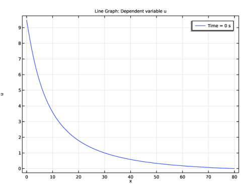
To model the initial condition, use the logical expression (x<40)*(40-x). This means that in the areas where x > 40, the initial value is zero.

COMSOL_Multiphysics/Equation_Based/black_scholes_put

Modeling Instructions

From the menu, choose .

In the window, click

.

1

In the window, click

.

2

In the tree, select > > .

3

4

5

In the tree, select > .

6

1

In the window, click the root node.

2

In the root node’s window, locate the section.

3

From the list, choose .

Keeping track of units is not important in this model; by turning off unit support, you avoid the need to specify dimensions for equation coefficients and coordinates to get rid of unit warnings.

Interval 1 (i1)

1

In the window, under right-click and choose .

2

In the window for , locate the section.

3

In the table, enter the following settings:


Coordinates
0
80

4

Global Definitions

1

In the window, under click .

2

In the window for , locate the section.

3

In the table, enter the following settings:


Name	Expression	Value	Description
r	0.12	0.12	Continuous compounding interest rate
sigma	0.3	0.3	Volatility

Coefficient Form PDE (c)

Coefficient Form PDE 1

1

In the window, under > click .

2

In the window for , locate the section.

3

In the c text field, type 1/2*sigma^2*x^2.

4

Locate the section. In the a text field, type r.

5

Locate the section. In the f text field, type 0.

6

Locate the section. In the da text field, type -1.

7

Click to expand the section. In the β text field, type (-r+sigma^2)*x.

Initial Values 1

1

In the window, click .

2

In the window for , locate the section.

3

In the u text field, type (x<40)*(40-x).

1

In the toolbar, click

and choose .

2

Select Boundary 1 only.

Dirichlet Boundary Condition 1

1

In the toolbar, click

and choose .

2

Select Boundary 2 only.

In the toolbar, click

.

1

In the window, click .

2

In the window for , locate the section.

3

Click the button.

4

Locate the section. In the text field, type 2.

5

The mesh consists of 40 elements.

Step 1: Time Dependent

1

In the window, under click .

2

In the window for , locate the section.

3

In the text field, type range(12,-0.5,0).

4

In the toolbar, click

.

To see the plot of u as a Line Graph at time = 0, follow the steps given below.

Coefficient Form PDE

1

In the window, under click .

2

In the window for , locate the section.

3

From the list, choose .

4

In the list box, select .

5

Click to expand the section. Locate the section.

6

Select the checkbox. In the associated text field, type x.

7

Select the checkbox. In the associated text field, type u.

1

In the window, expand the node, then click .

2

In the window for , click in the upper-right corner of the section. From the menu, choose > > > .

3

Click to expand the section. Select the checkbox.

4

Find the subsection. In the text field, type Time = .

5

In the toolbar, click

.