PDF

Molecular Flow Through a Microcapillary
Introduction
Computing molecular flows in arbitrary geometries produces complex integral equations which are very difficult to compute analytically. Analytic solutions are therefore only available for simple geometries. One of the earliest problems solved was that of gas flow through tubes of arbitrary length, which was first treated correctly by Clausing (Ref. 1). Later the integral expressions he derived were computed more accurately by Cole (Ref. 2). These authors derived values for the transmission probability of molecules incident on a tube of arbitrary length, which is independent of the pressure, provided that the Knudsen number is much greater than one (that is in the molecular flow regime).
This model uses COMSOL Multiphysics to compute the transmission probability for molecular flow of molecules through a microcapillary with different ratios of the length to the radius. The results are compared with the accurate solution due to Cole (Ref. 2).
Model Definition
Nitrogen gas flows through a microcapillary tube of diameter 200 μm, from a reservoir at a fixed pressure of 103 mBar to a reservoir at high vacuum. The flux of molecules entering the tube from the high vacuum end is assumed to be negligible. At this pressure the mean free path of the nitrogen is approximately 100 mm, so the Knudsen number of the flow is much greater than 1. The ratio of the flux of molecules entering the tube to the flux of molecules leaving the tube is computed for tube lengths of 0.4 mm, 0.8 mm, 1.2 mm, 1.6 mm, and 2.0 mm. The model is axially symmetric and is built in the 2D axially symmetric interface. The geometry is shown in Figure 1 for the case of the 2.0 mm long tube. The lower boundary is connected to the reservoir at low vacuum, the upper boundary is connected to the reservoir at high vacuum and the nonaxial vertical boundary is the capillary wall.
Figure 1: Model geometry.
The probability, χ, of molecules that strike the tube passing through the tube can be computed as the following integral:
where J is the outgoing flux, G is the incident flux, r is the radial distance, RS is the boundary adjacent to the reservoir, and HV is the boundary adjacent to high vacuum.
Results and Discussion
The incident flux on the surfaces of the tube is shown in Figure 2 for the case of the 2 mm long tube. A line plot of the pressure along the wall is shown in Figure 3. As expected, the incident flux decreases steadily from the reservoir end to the end at high vacuum, as does the pressure. Note that the incident flux (in contrast with the emitted flux) is not constant along the two reservoir boundaries, as it results from reflections within the geometry. The transmission probability for the tube is plotted against length to radius ratio in Figure 4. Good agreement is obtained between the calculated results and the probabilities calculated by Cole (Ref. 2).
Figure 2: The incident flux inside the tube.
Figure 3: The pressure along the tube wall.
Figure 4: The transmission probability for the pipe as a function of the length to radius ratio. The results due to Cole (Ref. 2) are shown for comparison.
Notes About the COMSOL Implementation
The model is straightforward to set up using the Molecular Flow interface. The capillary walls are assigned the wall boundary condition, the reservoir boundary condition is used for the bottom opening, and the top opening is assigned the total vacuum boundary condition. The geometry is parameterized, and a parametric solver is used to vary the capillary dimensions.
References
1. P. Clausing, “Über die Strömung sehr verdünnter Gase durch Röhren von beliebiger Länge,” Ann. Physik, vol. 404, no. 8, pp. 961–989, 1932. English translation available as: “The Flow of Highly Rarefied Gases Through Tubes of Arbitrary Length,” J. Vacuum Science and Technology, vol. 8. no. 5, pp. 636–646, 2009.
2. R.J. Cole, “Complementary Variational Principles for Knudsen Flow Rates,” IMA J. Appl. Math., vol. 20, pp. 107–115, 1977.
Application Library path: Molecular_Flow_Module/Benchmarks/vacuum_capillary
Modeling Instructions
From the File menu, choose New.
New
In the New window, click  Model Wizard.
Model Wizard
1
In the Model Wizard window, click  2D Axisymmetric.
2
In the Select Physics tree, select Fluid Flow > Rarefied Flow > Free Molecular Flow (fmf).
3
Click Add.
4
Click  Study.
5
In the Select Study tree, select General Studies > Stationary.
6
Global Definitions
Parameters 1
1
In the Model Builder window, under Global Definitions click Parameters 1.
2
In the Settings window for Parameters, locate the Parameters section.
3
Geometry 1
Rectangle 1 (r1)
1
In the Geometry toolbar, click  Rectangle.
2
In the Settings window for Rectangle, locate the Size and Shape section.
3
In the Width text field, type Rc.
4
In the Height text field, type Lc.
5
Click  Build All Objects.
6
Click the  Zoom Extents button in the Graphics toolbar.
Free Molecular Flow (fmf)
Set boundary conditions for the tube entrance and exit.
Total Vacuum 1
1
In the Physics toolbar, click  Boundaries and choose Total Vacuum.
2
Reservoir 1
1
In the Physics toolbar, click  Boundaries and choose Reservoir.
2
3
In the Settings window for Reservoir, locate the Reservoir section.
4
In the p0,G text field, type p0.
Definitions
Define an interpolation function for Cole’s solution for the transmission probability as a function of the length-to-radius ratio. You will use it later for comparison with the model result.
Interpolation 1 (int1)
1
In the Definitions toolbar, click  Interpolation.
2
In the Settings window for Interpolation, locate the Definition section.
3
Set up integration nonlocal couplings to compute the total flux of molecules through the system.
Integration 1 (intop1)
1
In the Definitions toolbar, click  Nonlocal Couplings and choose Integration.
2
In the Settings window for Integration, locate the Source Selection section.
3
From the Geometric entity level list, choose Boundary.
4
5
Locate the Advanced section. Clear the Compute integral in revolved geometry checkbox.
Integration 2 (intop2)
1
In the Definitions toolbar, click  Nonlocal Couplings and choose Integration.
2
In the Settings window for Integration, locate the Source Selection section.
3
From the Geometric entity level list, choose Boundary.
4
5
Locate the Advanced section. Clear the Compute integral in revolved geometry checkbox.
Use a mapped mesh for this simple geometry.
Mesh 1
Mapped 1
In the Mesh toolbar, click  Mapped.
Distribution 1
1
Right-click Mapped 1 and choose Distribution.
2
3
In the Settings window for Distribution, locate the Distribution section.
4
In the Number of elements text field, type 15.
Distribution 2
1
In the Model Builder window, right-click Mapped 1 and choose Distribution.
2
3
In the Settings window for Distribution, locate the Distribution section.
4
In the Number of elements text field, type 60.
5
Click  Build All.
Set up a parametric sweep over the capillary length.
Study 1
Parametric Sweep
1
In the Study toolbar, click  Parametric Sweep.
2
In the Settings window for Parametric Sweep, locate the Study Settings section.
3
4
From the list in the Parameter name column, choose Lc (Capillary length).
5
Click  Range.
6
In the Range dialog, type 0.4[mm] in the Start text field.
7
In the Stop text field, type 2[mm].
8
In the Step text field, type 0.4[mm].
9
Click Add.
10
In the Study toolbar, click  Compute.
Results
Incident Molecular Flux (fmf)
1
In the Settings window for 2D Plot Group, locate the Data section.
2
From the Parameter value (Lc (m)) list, choose 4E-4.
3
In the Incident Molecular Flux (fmf) toolbar, click  Plot.
4
Click the  Zoom Extents button in the Graphics toolbar.
The default plot shows the incident molecular flux inside the microcapillary tube. Compare with the plot in Figure 2.
Plot the pressure along the tube wall by following these steps.
Total Pressure
1
In the Results toolbar, click  1D Plot Group.
2
In the Settings window for 1D Plot Group, type Total Pressure in the Label text field.
3
Locate the Data section. From the Dataset list, choose Study 1/Parametric Solutions 1 (sol2).
4
From the Parameter selection (Lc) list, choose First.
Line Graph 1
1
Right-click Total Pressure and choose Line Graph.
2
3
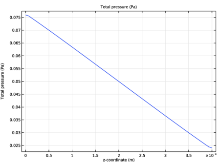
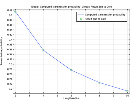
In the Settings window for Line Graph, click Replace Expression in the upper-right corner of the y-Axis Data section. From the menu, choose Component 1 (comp1) > Free Molecular Flow > Pressure > fmf.ptot - Total pressure - Pa.
4
Click to expand the Quality section. From the Evaluation settings list, choose Manual.
5
From the Resolution list, choose No refinement.
Use the z-coordinate for the x-axis data.
6
Locate the x-Axis Data section. From the Parameter list, choose Expression.
7
In the Expression text field, type z.
8
In the Total Pressure toolbar, click  Plot.
Compare the resulting plot with that in Figure 3.
Finally, plot the result for the transmission probability versus the length-to-radius ratio and compare with Cole’s solution.
1D Plot Group 5
1
In the Results toolbar, click  1D Plot Group.
2
In the Settings window for 1D Plot Group, locate the Data section.
3
From the Dataset list, choose Study 1/Parametric Solutions 1 (sol2).
Global 1
1
Right-click 1D Plot Group 5 and choose Global.
2
In the Settings window for Global, locate the y-Axis Data section.
3
4
Locate the x-Axis Data section. From the Parameter list, choose Expression.
5
In the Expression text field, type Lc/Rc.
Transmission Probability
1
In the Model Builder window, under Results click 1D Plot Group 5.
2
In the Settings window for 1D Plot Group, type Transmission Probability in the Label text field.
3
Locate the Plot Settings section.
4
Select the x-axis label checkbox. In the associated text field, type Length/radius.
5
Select the y-axis label checkbox. In the associated text field, type Transmission probability.
Global 2
1
Right-click Transmission Probability and choose Global.
2
In the Settings window for Global, locate the y-Axis Data section.
3
4
Locate the x-Axis Data section. From the Parameter list, choose Expression.
5
In the Expression text field, type Lc/Rc.
Change the plot style to display only the data points.
6
Click to expand the Coloring and Style section. Find the Line style subsection. From the Line list, choose None.
7
Find the Line markers subsection. From the Marker list, choose Square.
Transmission Probability
1
In the Model Builder window, click Transmission Probability.
2
In the Transmission Probability toolbar, click  Plot.
Compare with Figure 4.