PDF

Ultrahigh Vacuum, Chemical Vapor Deposition
Introduction
Chemical vapor deposition (CVD) is a process often used in the semiconductor industry for epitaxial layer growth of high-purity silicon on top of a wafer substrate.
CVD is achieved using many different techniques and across a range of pressures; however, of particular commercial interest is the multilayer ultrahigh vacuum (UHV)/CVD technique.
UHV/CVD is performed at pressures below 106 Pa (108 Torr), so gas transport is achieved by molecular flow and lacks any hydrodynamic effects such as boundary layers. In addition, there is also no gas-phase chemistry involved due to the low frequency of molecular collisions, so growth rate will be determined by the number density of species and surface molecular decomposition processes.
Model Definition
Typically wafers are arranged close together (relative to their diameters) on a movable wafer boat within a quartz tube, surrounded by a furnace. Reactant gases are introduced at one end via a load lock together with a dilution gas such as hydrogen. A turbopump is present at the other end of the quartz tube.
The model geometry is shown in Figure 1. The wafer cassette is positioned within the quartz chamber by means of a delivery rail.
Figure 1: Model geometry. Key components of the system are labeled.
The reactant gas, silane (SiH4) along with a dilution gas, hydrogen (H2) enters through the inlet. The total gas mass flow rate is 1 SCCM (0.2 SCCM SiH4, 0.8 SCCM H2). The outgassing wall boundary condition is used for this inlet.
A vacuum pump is positioned at the other end of the chamber at the cylindrical port. Three different pumping curves are investigated for both the hydrogen and the silane. These pumping curves are loaded into COMSOL Multiphysics as interpolations functions and are switched between using a sweep parameter that will allow us to run the model for each curve.
All other surfaces in the model are walls.
Results and Discussion
The molecular flux fraction of SiH4 at the wafer cassette, using pumping curves 2, is shown in Figure 2. The interesting result is that the molecular flux fraction of silane at the wafer cassette is significantly different from what is introduced at the inlet. As this directly controls the growth on the wafers, the choice of pump seems to be important. In addition, this molecular flux fraction cannot easily be measures at the wafer so its important to use models like this to investigate the process fully.
Figure 2: Molecular flux fraction of SiH4 at the water cassette.
Reference
1. B. S. Meyerson, Appl. Phys. Lett. 48, pp. 797–799, 1986.
Application Library path: Molecular_Flow_Module/Industrial_Applications/uhv_cvd
Modeling Instructions
From the File menu, choose New.
New
In the New window, click  Model Wizard.
Model Wizard
1
In the Model Wizard window, click  3D.
2
In the Select Physics tree, select Fluid Flow > Rarefied Flow > Free Molecular Flow (fmf).
3
Click Add.
4
Click  Study.
5
In the Select Study tree, select General Studies > Stationary.
6
Global Definitions
Parameters 1
1
In the Model Builder window, under Global Definitions click Parameters 1.
2
In the Settings window for Parameters, locate the Parameters section.
3
Click  Load from File.
4
Geometry 1
The geometry consists of a cylindrical chamber with an inlet and vacuum pump at either end. A cassette of silicon wafers is approximated by a cylinder of narrower diameter on the end of a delivery rail.
Cylinder 1 (cyl1)
1
In the Geometry toolbar, click  Cylinder.
2
In the Settings window for Cylinder, locate the Size and Shape section.
3
In the Radius text field, type R0.
4
In the Height text field, type L0.
5
Locate the Position section. In the x text field, type -Lo/2.
6
Locate the Axis section. From the Axis type list, choose x-axis.
7
Locate the Position section. In the x text field, type -L0/2.
Cylinder 2 (cyl2)
1
In the Geometry toolbar, click  Cylinder.
2
In the Settings window for Cylinder, locate the Size and Shape section.
3
In the Radius text field, type Dp/2.
4
In the Height text field, type Dp/4+R0.
5
Locate the Position section. In the x text field, type 0.3*L0.
6
In the z text field, type -(R0+Dp/4).
Union 1 (uni1)
1
In the Geometry toolbar, click  Booleans and Partitions and choose Union.
2
Click in the Graphics window and then press Ctrl+A to select both objects.
3
In the Settings window for Union, locate the Union section.
4
Clear the Keep interior boundaries checkbox.
Cylinder 3 (cyl3)
1
In the Geometry toolbar, click  Cylinder.
2
In the Settings window for Cylinder, locate the Size and Shape section.
3
In the Radius text field, type Dw/2.
4
In the Height text field, type Lw.
5
Locate the Position section. In the x text field, type -Lw/2.
6
Locate the Axis section. From the Axis type list, choose x-axis.
Cylinder 4 (cyl4)
1
In the Geometry toolbar, click  Cylinder.
2
In the Settings window for Cylinder, locate the Size and Shape section.
3
In the Radius text field, type Dw/10.
4
In the Height text field, type L0/2.
5
Locate the Axis section. From the Axis type list, choose x-axis.
Union 2 (uni2)
1
In the Geometry toolbar, click  Booleans and Partitions and choose Union.
2
Click the  Wireframe Rendering button in the Graphics toolbar.
3
Select the objects cyl3 and cyl4 only.
4
In the Settings window for Union, locate the Union section.
5
Clear the Keep interior boundaries checkbox.
Difference 1 (dif1)
1
In the Geometry toolbar, click  Booleans and Partitions and choose Difference.
2
3
In the Settings window for Difference, locate the Difference section.
4
Click to select the  Activate Selection toggle button for Objects to subtract.
5
Cylinder 5 (cyl5)
1
In the Geometry toolbar, click  Cylinder.
2
In the Settings window for Cylinder, locate the Size and Shape section.
3
In the Radius text field, type Rin.
4
In the Height text field, type 1.5*(R0).
5
Locate the Position section. In the x text field, type -0.9*L0/2.
6
In the y text field, type -1.5*R0.
7
Locate the Axis section. From the Axis type list, choose y-axis.
Difference 2 (dif2)
1
In the Geometry toolbar, click  Booleans and Partitions and choose Difference.
2
3
In the Settings window for Difference, locate the Difference section.
4
Click to select the  Activate Selection toggle button for Objects to subtract.
5
6
Select the Keep objects to subtract checkbox.
7
Click  Build All Objects.
Definitions
Set up some selections to assist during postprocessing.
Cassette
1
In the Definitions toolbar, click  Explicit.
2
In the Settings window for Explicit, locate the Input Entities section.
3
From the Geometric entity level list, choose Boundary.
4
5
In the Label text field, type Cassette.
Cassette and rail
1
In the Definitions toolbar, click  Explicit.
2
In the Settings window for Explicit, locate the Input Entities section.
3
From the Geometric entity level list, choose Boundary.
4
5
In the Label text field, type Cassette and rail.
Interpolation 1 (int1)
1
In the Definitions toolbar, click  Interpolation.
2
In the Settings window for Interpolation, locate the Definition section.
3
Click  Load from File.
4
5
In the Function name text field, type pump1_H2.
6
Locate the Units section. In the Argument table, enter the following settings:
7
In the Function table, enter the following settings:
Interpolation 2 (int2)
1
In the Definitions toolbar, click  Interpolation.
2
In the Settings window for Interpolation, locate the Definition section.
3
Click  Load from File.
4
5
In the Function name text field, type pump2_H2.
6
Locate the Units section. In the Argument table, enter the following settings:
7
In the Function table, enter the following settings:
Interpolation 3 (int3)
1
In the Definitions toolbar, click  Interpolation.
2
In the Settings window for Interpolation, locate the Definition section.
3
Click  Load from File.
4
5
In the Function name text field, type pump3_H2.
6
Locate the Units section. In the Argument table, enter the following settings:
7
In the Function table, enter the following settings:
Interpolation 4 (int4)
1
In the Definitions toolbar, click  Interpolation.
2
In the Settings window for Interpolation, locate the Definition section.
3
Click  Load from File.
4
5
In the Function name text field, type pump1_SiH4.
6
Locate the Units section. In the Argument table, enter the following settings:
7
In the Function table, enter the following settings:
Interpolation 5 (int5)
1
In the Definitions toolbar, click  Interpolation.
2
In the Settings window for Interpolation, locate the Definition section.
3
Click  Load from File.
4
5
In the Function name text field, type pump2_SiH4.
6
Locate the Units section. In the Argument table, enter the following settings:
7
In the Function table, enter the following settings:
Interpolation 6 (int6)
1
In the Definitions toolbar, click  Interpolation.
2
In the Settings window for Interpolation, locate the Definition section.
3
Click  Load from File.
4
5
In the Function name text field, type pump3_SiH4.
6
Locate the Units section. In the Argument table, enter the following settings:
7
In the Function table, enter the following settings:
Set up two species, silane (SiH4) and hydrogen (H2) as a dilution gas.
Free Molecular Flow (fmf)
1
In the Model Builder window, under Component 1 (comp1) click Free Molecular Flow (fmf).
2
In the Settings window for Free Molecular Flow, click to expand the Dependent Variables section.
3
In the Number of species text field, type 2.
4
In the Incident molecular fluxes (1/(m²·s)) table, enter the following settings:
5
Locate the Compute section. Clear the Number density checkbox.
Specify the molecular weights for both species.
Molecular Flow 1
1
In the Model Builder window, under Component 1 (comp1) > Free Molecular Flow (fmf) click Molecular Flow 1.
2
In the Settings window for Molecular Flow, locate the Molecular Weight of Species section.
3
In the Mn,H2 text field, type 2[g/mol].
4
In the Mn,SiH4 text field, type 32.12[g/mol].
Set the temperature of the surrounding furnace.
Surface Temperature 1
1
In the Model Builder window, click Surface Temperature 1.
2
In the Settings window for Surface Temperature, locate the Surface Temperature section.
3
In the T text field, type Tf.
Add an outgassing wall to the inlet with the mass flows of each species.
Wall 2
1
In the Physics toolbar, click  Boundaries and choose Wall.
2
3
In the Settings window for Wall, locate the Wall Type section.
4
From the Wall type list, choose Outgassing wall.
5
Locate the Flux section. From the Outgoing flux list, choose Number of SCCM units.
6
In the Qsccm,H2 text field, type sccmH2.
7
In the Qsccm,SiH4 text field, type sccmSiH4.
Add a vacuum pump and specify the pump speed for each species.
Vacuum Pump 1
1
In the Physics toolbar, click  Boundaries and choose Vacuum Pump.
2
3
In the Settings window for Vacuum Pump, locate the Vacuum Pump section.
4
From the Specify pump flux list, choose Pump speed.
5
In the SH2 text field, type pump1_H2(fmf.ptot)*(sp==1)+pump2_H2(fmf.ptot)*(sp==2)+pump3_H2(fmf.ptot)*(sp==3).
6
In the SSiH4 text field, type pump1_SiH4(fmf.ptot)*(sp==1)+pump2_SiH4(fmf.ptot)*(sp==2)+pump3_SiH4(fmf.ptot)*(sp==3).
Add a surface mesh.
Mesh 1
Free Triangular 1
1
In the Mesh toolbar, click  More Generators and choose Free Triangular.
2
In the Settings window for Free Triangular, locate the Boundary Selection section.
3
From the Selection list, choose Cassette and rail.
Size 1
1
Right-click Free Triangular 1 and choose Size.
2
In the Settings window for Size, locate the Element Size section.
3
From the Predefined list, choose Extra fine.
Free Triangular 2
1
In the Mesh toolbar, click  More Generators and choose Free Triangular.
2
In the Settings window for Free Triangular, locate the Boundary Selection section.
3
From the Geometric entity level list, choose Remaining.
Size
1
In the Model Builder window, click Size.
2
In the Settings window for Size, locate the Element Size section.
3
From the Predefined list, choose Finer.
Add two average nonlocal couplings to allow the evaluation of properties on and around the wafer cassette and vacuum pump.
Definitions
Average 1 (aveop1)
1
In the Definitions toolbar, click  Nonlocal Couplings and choose Average.
2
In the Settings window for Average, locate the Source Selection section.
3
From the Geometric entity level list, choose Boundary.
4
From the Selection list, choose Cassette.
Average 2 (aveop2)
1
In the Definitions toolbar, click  Nonlocal Couplings and choose Average.
2
In the Settings window for Average, locate the Source Selection section.
3
From the Geometric entity level list, choose Boundary.
4
Set the study up to cover a range of inlet mass flows for pump 1, 2, and 3.
Study 1
Step 1: Stationary
1
In the Model Builder window, under Study 1 click Step 1: Stationary.
2
In the Settings window for Stationary, click to expand the Study Extensions section.
3
Select the Auxiliary sweep checkbox.
4
5
6
In the Study toolbar, click  Compute.
Results
Study 1/Solution 1 (2) (sol1)
1
In the Model Builder window, expand the Results > Datasets node.
2
Right-click Results > Datasets > Study 1/Solution 1 (sol1) and choose Duplicate.
Selection
1
In the Results toolbar, click  Attributes and choose Selection.
2
In the Settings window for Selection, locate the Geometric Entity Selection section.
3
From the Geometric entity level list, choose Boundary.
4
From the Selection list, choose Cassette and rail.
Add a Global Evaluation node to evaluate the molecular flux of SiH4 and molecular flux fraction of SiH4 at the position of the cassette, as well as the average pressure at the vacuum pump.
Global Evaluation 1
1
In the Results toolbar, click  Global Evaluation.
2
In the Settings window for Global Evaluation, locate the Expressions section.
3
4
Click  Evaluate.
Molecular Flux Fraction SiH4
1
In the Results toolbar, click  3D Plot Group.
2
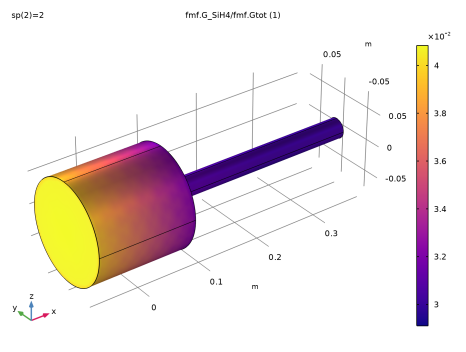
In the Settings window for 3D Plot Group, type Molecular Flux Fraction SiH4 in the Label text field.
3
Locate the Data section. From the Dataset list, choose Study 1/Solution 1 (2) (sol1).
4
From the Parameter value (sp) list, choose 2.
Surface 1
1
Right-click Molecular Flux Fraction SiH4 and choose Surface.
2
In the Settings window for Surface, locate the Expression section.
3
In the Expression text field, type fmf.G_SiH4/fmf.Gtot.
4
Locate the Coloring and Style section. From the Color table list, choose Plasma.
5
In the Molecular Flux Fraction SiH4 toolbar, click  Plot.