
|
|
|













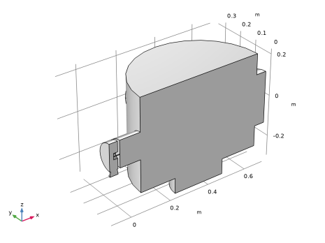
|
1
|
|
2
|
|
3
|
Click Add.
|
|
4
|
Click
 Study. Study. |
|
5
|
|
6
|
Click
 Done. Done. |
|
1
|
|
2
|
Browse to the model’s Application Libraries folder and double-click the file differential_pumping_geom_sequence.mph.
|
|
3
|
|
4
|
|
1
|
|
2
|
|
3
|
Click
 Load from File. Load from File. |
|
4
|
Browse to the model’s Application Libraries folder and double-click the file differential_pumping_parameters.txt.
|
|
5
|
Click the
 Wireframe Rendering button in the Graphics toolbar. Wireframe rendering enables easier visualization of the interior boundaries. Wireframe Rendering button in the Graphics toolbar. Wireframe rendering enables easier visualization of the interior boundaries. |
|
1
|
|
2
|
|
3
|
|
1
|
|
2
|
|
3
|
Click
 Load from File. Load from File. |
|
4
|
Browse to the model’s Application Libraries folder and double-click the file differential_pumping_variables.txt.
|
|
1
|
|
2
|
|
3
|
|
4
|
|
5
|
|
1
|
In the Model Builder window, under Component 1 (comp1) > Free Molecular Flow (fmf) click Molecular Flow 1.
|
|
2
|
|
3
|
|
1
|
|
2
|
|
3
|
|
1
|
|
2
|
|
3
|
|
4
|
|
5
|
|
1
|
|
2
|
|
3
|
|
4
|
|
5
|
|
6
|
|
1
|
|
1
|
|
2
|
|
3
|
|
4
|
|
5
|
|
1
|
|
2
|
|
3
|
|
1
|
|
2
|
|
3
|
|
4
|
Click
 Build All. Build All. |
|
1
|
|
2
|
|
3
|
Select the Auxiliary sweep checkbox.
|
|
4
|
Click
 Add. Add. |
|
6
|
|
1
|
In the Model Builder window, expand the Results > Datasets node, then click Study 1/Solution 1 (sol1).
|
|
1
|
|
2
|
|
3
|
|
4
|
|
1
|
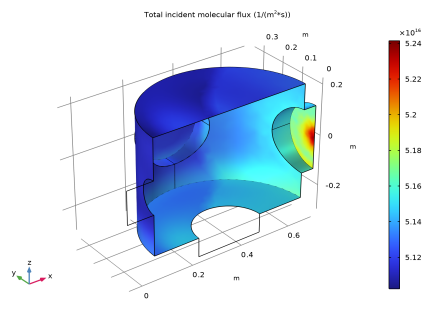
In the Model Builder window, expand the Results > Incident Molecular Flux (fmf) node, then click Surface.
|
|
2
|
|
3
|
|
1
|
|
2
|
|
3
|
|
1
|
|
2
|
|
1
|
|
2
|
|
4
|
|
5
|
|
6
|
|
7
|
Click to expand the Coloring and Style section. Find the Line markers subsection. From the Marker list, choose Circle.
|
|
8
|
|
9
|
|
10
|
|
1
|
|
2
|
|
3
|
|
4
|
Locate the Plot Settings section.
|
|
5
|
|
1
|
|
2
|
|
4
|
|
5
|
|
6
|
|
7
|
|
8
|
Locate the Coloring and Style section. Find the Line markers subsection. From the Marker list, choose Diamond.
|
|
1
|
|
2
|
|
3
|
|
1
|
|
2
|
|
4
|
Click
 Evaluate. Evaluate. |
|
1
|
Go to the Table 1 window.
|
|
1
|
|
2
|
Go to the Add Physics window.
|
|
3
|
|
4
|
Find the Physics interfaces in study subsection. In the table, clear the Solve checkbox for Study 1.
|
|
5
|
Click the Add to Component 1 button in the window toolbar.
|
|
6
|
|
1
|
|
2
|
Go to the Add Study window.
|
|
3
|
|
4
|
Click the Add Study button in the window toolbar.
|
|
5
|
|
2
|
|
3
|
Clear the Pressure checkbox.
|
|
4
|
|
1
|
In the Model Builder window, under Component 1 (comp1) > Free Molecular Flow 2 (fmf2) click Molecular Flow 1.
|
|
2
|
|
3
|
|
1
|
|
2
|
|
3
|
|
1
|
|
2
|
|
3
|
|
4
|
|
5
|
|
1
|
|
2
|
|
3
|
|
4
|
|
1
|
|
2
|
|
3
|
|
4
|
|
1
|
|
2
|
|
3
|
Click
 Clear Selection. Clear Selection. |
|
4
|
|
1
|
|
1
|
|
2
|
|
3
|
|
4
|
|
5
|
|
6
|
|
1
|
|
2
|
|
3
|
|
1
|
|
2
|
|
3
|
|
4
|
|
5
|
|
6
|
|
1
|
|
2
|
|
3
|
|
4
|
Click
 Build Selected. Build Selected. |
|
1
|
|
2
|
|
3
|
|
1
|
|
2
|
|
3
|
|
1
|
|
2
|
|
3
|
|
1
|
|
3
|
|
1
|
|
2
|
|
3
|
In the Solve for column of the table, under Component 1 (comp1), clear the checkbox for Free Molecular Flow (fmf).
|
|
4
|
Click to expand the Mesh Selection section. In the table, enter the following settings:
|
|
5
|
|
1
|
|
2
|
|
3
|
|
4
|
|
1
|
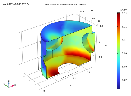
In the Model Builder window, expand the Results > Incident Molecular Flux (fmf2) node, then click Surface.
|
|
2
|
|
1
|
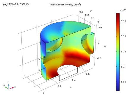
In the Model Builder window, expand the Results > Total Number Density (fmf2) node, then click Surface.
|
|
2
|
|
1
|
|
2
|
|
3
|
|
4
|
Locate the Plot Settings section.
|
|
5
|
|
6
|
Select the y-axis label checkbox. In the associated text field, type number density (1/m<sup>3</sup>).
|
|
7
|
|
8
|
|
9
|
|
1
|
|
3
|
|
4
|
|
5
|
|
6
|
|
7
|
|
1
|
|
2
|
|
4
|
|
5
|
|
6
|
Locate the Coloring and Style section. Find the Line style subsection. From the Line list, choose None.
|
|
7
|
|
8
|
|
9
|
|
1
|
|
2
|
|
4
|
|
5
|
|
6
|
|
7
|
Locate the Coloring and Style section. Find the Line style subsection. From the Line list, choose None.
|
|
8
|
|
9
|
|
1
|
|
2
|
|
3
|
|
4
|
Locate the Expressions section. In the table, enter the following settings:
|
|
5
|
Click
 Evaluate. Evaluate. |
|
1
|
|
2
|
|
4
|
|
1
|
|
2
|
|
4
|
|
1
|
Go to the Table 2 window.
|
|
1
|
|
2
|
|
3
|
|
4
|
|
5
|
|
6
|
|
1
|
|
2
|
|
3
|
|
4
|
|
5
|
|
6
|
|
7
|
Locate the Axis section. From the Axis type list, choose y-axis. By changing the axis, the cylinder is oriented accordingly.
|
|
1
|
|
2
|
|
3
|
|
4
|
|
5
|
|
6
|
|
1
|
|
2
|
|
3
|
|
4
|
|
5
|
|
6
|
|
1
|
|
2
|
|
3
|
|
4
|
|
5
|
|
6
|
|
1
|
|
2
|
|
3
|
|
4
|
Clear the Keep interior boundaries checkbox. This combines the selected cylinders into an object with a single domain.
|
|
1
|
|
2
|
|
3
|
|
4
|
|
5
|
|
6
|
|
1
|
|
2
|
|
3
|
|
4
|
|
5
|
|
6
|
|
7
|
|
1
|
|
2
|
|
3
|
|
4
|
Clear the Keep interior boundaries checkbox.
|
|
1
|
|
2
|
|
3
|
|
4
|
|
5
|
|
6
|
|
1
|
|
2
|
Select the object uni2 only.
|
|
3
|
|
4
|
|
5
|
Select the object cyl7 only.
|
|
1
|
|
2
|
|
3
|
|
4
|
|
5
|
|
6
|
|
1
|
|
2
|
|
3
|
|
1
|
|
2
|
Click in the Graphics window and then press Ctrl+A to select all objects.
|
|
3
|
|
4
|
|
1
|
|
2
|
|
3
|
|
4
|
|
5
|
On the object par1(1), select Domain 1 only.
|
|
6
|
On the object par1(2), select Domain 1 only.
|
|
7
|
On the object par1(3), select Domain 1 only.
|
|
8
|
Click
 Build Selected. Build Selected. |
|
1
|
|
2
|
|
1
|
|
2
|
|
3
|
On the object fin, select Domain 3 only.
|
|
1
|
|
2
|
|
3
|
|
4
|
|
5
|
Click OK.
|
|
1
|
|
2
|
|
3
|
|
4
|
|
5
|
On the object fin, select Boundary 19 only.
|
|
1
|
|
2
|
|
3
|
|
4
|
|
5
|
|
6
|
Click OK.
|
|
7
|
|
8
|
|
9
|
|
10
|
Click OK.
|
|
1
|
|
2
|
|
3
|
|
4
|
On the object fin, select Boundary 9 only.
|
|
1
|
|
2
|
|
3
|
|
4
|
Select the Group by continuous tangent checkbox.
|
|
5
|
On the object fin, select Boundaries 11 and 12 only.
|
|
1
|
|
2
|
|
3
|
|
4
|
On the object fin, select Boundary 25 only.
|
|
1
|
|
2
|
|
3
|
|
4
|
On the object fin, select Boundary 35 only.
|
|
1
|
|
2
|
|
3
|
|
4
|
|
5
|
|
1
|
|
2
|
|
3
|
|
4
|
|
5
|
|
6
|
|
1
|
|
2
|
|
3
|
|
4
|
|
5
|
|
6
|
|
1
|
|
2
|
|
3
|
|
4
|
|
5
|
|
6
|
Click OK.
|
|
7
|
|
8
|
|
9
|
In the Add dialog, in the Selections to subtract list, choose Cylinder Selection 1 and Cylinder Selection 2.
|
|
10
|
Click OK.
|


 next to
 next to


