PDF

Mixing of Water in a Flat Bottom Mixer
Introduction
This model simulates the flow in a flat bottom mixer agitated by a pitched four blade impeller. The mixed fluid is water, and the flow is assumed turbulent due to the significant mixer Reynolds number (5.33·104). The flow is modeled using the k-ε turbulence model, and a time-dependent simulation corresponding to 34 revolutions of the impeller is performed in order to reach the operating conditions of the mixer.
When postprocessing the results, the self-similarity of the axial flow along the baffles is analyzed. In agreement with Ref. 1, the normalized velocity profiles at different axial positions are found to be self-similar indicating that the flow in this region resembles a three dimensional wall jet.
Model Definition
The mixer simulated consists of a baffled flat-bottom vessel and a pitched four-blade impeller. The mixer geometry and the simulation conditions used in this model correspond to the ones used in the experiments of Bittorf and Kresta (Ref. 1). The height (H) and diameter (T) of the mixer vessel is 0.24 m. The diameter of the impeller, Da, is 0.33T, and the clearance, C, between the impeller and the bottom is 0.40Da. The pitch of the impeller blades is 45°. The geometry of the mixer simulated is shown in Figure 1. The fluid contained in the mixer is water, which is mixed using an impeller rotational frequency of N = 8.58 turns per second. The resulting impeller Reynolds number is:
(1)
where μ and ρ are the dynamic viscosity (SI unit: kg/(m·s)) and density (SI unit: kg/m3) of water, respectively. The impeller Reynolds number is significantly higher than one, and the resulting flow will be treated as turbulent. The turbulent flow is modeled using the k-ε turbulence model, and the time-dependent problem is solved for 34 revolutions of the impeller.
Figure 1: Mixer geometry showing the vessel, baffles, and impeller.
Wall Jet Flow
Bittorf and Kresta (Ref. 1) compared the flow at the wall of a stirred tank to that of a turbulent wall jet. They found that the flow along the baffles of the stirred tank compares well to a three-dimensional wall jet. In order to assess whether the flow in this region of the mixer has the characteristics of a wall jet, the self-similarity of the axial velocity profiles can be examined. Self-similarity implies that the mean velocity profiles can be collapsed onto a single profile when scaled with properly chosen length and velocity scales. The existence of self-similarity indicates that the turbulent time scale is small enough for the turbulence to adjust locally to the development of the jet.
For wall jets, the spreading is typically found to be characterized by the maximum jet velocity, Um, and the distance from the wall to the position where the local velocity is equal to half of the maximum velocity value. The latter is often referred to as the jet half width and denoted by y1/2. Using the velocity data in Ref. 1, a similarity profile for a wall jet in a recirculating flow was suggested by Bhattacharya and Kresta in Ref. 2:
(2)
Here η denotes the distance from the wall normalized by the half width, η = y/y1/2. When analyzing the results, the self-similarity will be assessed by plotting the normalized axial velocity along the line shown in Figure 2. This corresponds to the position used in Ref. 1.
Figure 2: Measurement position for analyzing the self-similarity of the axial velocity profiles.
Solution Procedure
In order to minimize the time required to reach a fully developed, yet transient, flow state, the model is solved in two steps. First, a Frozen Rotor study is used to reach a good initial solution without having to solve the startup of the problem. In order to converge this step, a parametric sweep is used to first solve the model with a low Reynolds number and increased dynamic viscosity, and then compute it again with the actual dynamic viscosity of the fluid.
The frozen rotor solution is then used as initial condition for the transient simulation. During the transient simulation the model is run for 4.0 s corresponding to 34 full revolutions of the impeller.
Time averaging
An Identity Mapping nonlocal coupling is used when computing time-averaged velocity profiles. This is done to make sure that the average is computed along the measurement positions shown Figure 2, regardless of the position of the rotating impeller domain. The averages are computed using the time average operator in the manner of
timeavg(3.5,4,idmap1(w),'nointerp')
where the axial velocity is averaged between t = 3.5  and 4 s. The nointerp flag is used to compute the average without applying interpolation between the stored time steps.
Results and Discussion
The resulting flow field in the mixer after 4.0 s of transient simulation is shown in Figure 3. The streamlines show how the impeller pumps fluid downward along the shaft and ejects it toward the bottom of the vessel. The maximum velocity magnitude occurs at the tip of the impeller blades.
The velocity magnitude in a single cross section including the velocity vectors is shown in Figure 4. From this figure the main flow structure of the mixer can be further examined. The fluid flows with high speed along the bottom of the mixer. Upon reaching the wall, vertical high speed streaks form along the outer walls, and the fluid velocity decreases toward the top of the vessel. Fluid at the top of the vessel travel toward the impeller shaft prior to becoming pumped down toward the impeller.
Figure 3: Fluid flow at t = 4.0 s. The color of the slice plots and the width of the streamlines indicate the velocity magnitude.
Figure 4: Fluid flow magnitude and direction, at t = 4.0 s, in a cross section of the mixer.
The characteristics of the upward flow along the outer walls is studied in Figure 5 to analyze the wall jet. The averaged axial velocity, measured along the line shown in Figure 2, is plotted at different heights from the vessel bottom. The lines correspond to z/T equal to 0.458, 0.563, 0.667, and 0.771. The fluid velocity profiles are scaled by their individual maximum velocity, and the distance from the wall is normalized by the jet half width as defined in the section Wall Jet Flow. The similarity solution of Bhattacharya and Kresta (Equation 2) is also plotted.
The scaled velocity profiles are found to collapse on top of the similarity solution, at least for the first three positions from the bottom. The collapse occurs for η < 1.5; further out from the wall, the velocity is directed in the opposite direction, corresponding to the downward flow along the impeller shaft as seen in Figure 3 and Figure 4. The collapse in the region with upward flow indicates that the flow along the outer walls does indeed correspond to a wall jet flow. The results in Figure 5 compare well with the experimental results in Ref. 1.
Figure 5: Normalized axial velocity profiles measured at increasing mixer heights.
References
1. K.J. Bittorf and S.M. Kresta, “Three-dimensional wall jets: axial flow in a stirred tank,” AIChE Journal, vol. 47, no. 6, pp. 1277–1284, 2001.
2. S. Bhattacharya and S.M. Kresta, “CFD Simulations of Three-dimensional Wall Jets in a Stirred Tank,” Can. J. Chem. Eng., vol. 80, no. 4, pp. 1–15, 2002.
Application Library path: Mixer_Module/Benchmarks/wall_jet_4PB_mixer_flat
Modeling Instructions
From the File menu, choose New.
New
In the New window, click  Model Wizard.
Model Wizard
1
In the Model Wizard window, click  3D.
2
In the Select Physics tree, select Fluid Flow > Single-Phase Flow > Rotating Machinery, Fluid Flow > Turbulent Flow > Turbulent Flow, k-ε.
3
Click Add.
4
Click  Study.
5
In the Select Study tree, select Preset Studies for Selected Physics Interfaces > Frozen Rotor.
6
Geometry 1
Load the parameterized geometry sequence from file.
1
In the Geometry toolbar, click Insert Sequence and choose Insert Sequence.
2
3
In the Geometry toolbar, click  Build All.
Global Definitions
Parameters 1
1
In the Model Builder window, under Global Definitions click Parameters 1.
2
In the Settings window for Parameters, locate the Parameters section.
3
Moving Mesh
Rotating Domain 1
1
Click the  Zoom Extents button in the Graphics toolbar.
2
In the Model Builder window, under Component 1 (comp1) > Moving Mesh click Rotating Domain 1.
3
In the Settings window for Rotating Domain, locate the Domain Selection section.
4
5
Click  Remove from Selection.
6
7
Locate the Rotation section. In the f text field, type -N0.
Definitions
Identity Mapping 1 (idmap1)
1
In the Definitions toolbar, click  Nonlocal Couplings and choose Identity Mapping.
2
In the Settings window for Identity Mapping, locate the Source Selection section.
3
From the Selection list, choose All domains.
4
Locate the Frames section. From the Destination frame list, choose Material  (X, Y, Z).
Materials
Add water from the Material Library.
Add Material
1
In the Materials toolbar, click  Add Material to open the Add Material window.
2
Go to the Add Material window.
3
In the tree, select Built-in > Water, liquid.
4
Right-click and choose Add to Component 1 (comp1).
5
In the Materials toolbar, click  Add Material to close the Add Material window.
Materials
Water, liquid (mat1)
1
In the Settings window for Material, locate the Material Contents section.
2
Turbulent Flow, k-ε (spf)
Pressure Point Constraint 1
1
In the Physics toolbar, click  Points and choose Pressure Point Constraint.
2
Symmetry 1
1
In the Physics toolbar, click  Boundaries and choose Symmetry.
2
Interior Wall 1
1
In the Physics toolbar, click  Boundaries and choose Interior Wall.
2
Click the  Wireframe Rendering button in the Graphics toolbar.
3
Interior Wall 2
1
In the Physics toolbar, click  Boundaries and choose Interior Wall.
2
Mesh 1
1
In the Model Builder window, under Component 1 (comp1) click Mesh 1.
2
In the Settings window for Mesh, locate the Physics-Controlled Mesh section.
3
In the table, clear the Use checkbox for Geometric Analysis, Detail Size.
4
From the Element size list, choose Coarser.
5
Locate the Sequence Type section. From the list, choose User-controlled mesh.
Size 1
1
In the Model Builder window, under Component 1 (comp1) > Mesh 1 click Size 1.
2
In the Settings window for Size, locate the Element Size section.
3
Click the Custom button.
4
Locate the Element Size Parameters section. Select the Maximum element size checkbox.
5
Select the Minimum element size checkbox.
6
In the Maximum element size text field, type 0.01.
Size 2
1
In the Model Builder window, right-click Mesh 1 and choose Size.
2
In the Settings window for Size, locate the Geometric Entity Selection section.
3
From the Geometric entity level list, choose Domain.
4
From the Selection list, choose Tank (Pitched Blade Impeller 1).
5
6
Locate the Element Size section. From the Predefined list, choose Fine.
7
Click the Custom button.
8
Locate the Element Size Parameters section.
9
Select the Maximum element size checkbox. In the associated text field, type 0.008.
10
Select the Minimum element size checkbox. In the associated text field, type 0.001.
11
Right-click Size 2 and choose Move Up three times.
Free Tetrahedral 1
1
In the Model Builder window, click Free Tetrahedral 1.
2
In the Settings window for Free Tetrahedral, locate the Domain Selection section.
3
From the Geometric entity level list, choose Domain.
4
5
In the Model Builder window, right-click Mesh 1 and choose Build All.
Study 1
Step 1: Frozen Rotor
Set up an auxiliary continuation sweep for the visc_fact parameter.
1
In the Model Builder window, under Study 1 click Step 1: Frozen Rotor.
2
In the Settings window for Frozen Rotor, click to expand the Study Extensions section.
3
Select the Auxiliary sweep checkbox.
4
5
6
From the Run continuation for list, choose No parameter.
7
From the Reuse solution from previous step list, choose Yes.
8
In the Model Builder window, click Study 1.
9
In the Settings window for Study, locate the Study Settings section.
10
Clear the Generate default plots checkbox.
11
In the Study toolbar, click  Compute.
Now run a time-dependent simulation using the results from the frozen rotor study as initial values.
Definitions
Identity Boundary Pair 1 (ap1)
1
In the Model Builder window, under Component 1 (comp1) > Definitions click Identity Boundary Pair 1 (ap1).
2
In the Settings window for Pair, locate the Advanced section.
3
From the Elementwise mapping for compatible meshes list, choose Off.
Add Study
1
In the Home toolbar, click  Add Study to open the Add Study window.
2
Go to the Add Study window.
3
Find the Studies subsection. In the Select Study tree, select General Studies > Time Dependent.
4
Click the Add Study button in the window toolbar.
5
In the Home toolbar, click  Add Study to close the Add Study window.
Study 2
Step 1: Time Dependent
1
In the Settings window for Time Dependent, locate the Study Settings section.
2
In the Output times text field, type range(0,0.2,3), range(3, 0.05, 4).
3
Click to expand the Values of Dependent Variables section. Find the Initial values of variables solved for subsection. From the Settings list, choose User controlled.
4
From the Method list, choose Solution.
5
From the Study list, choose Study 1, Frozen Rotor.
6
From the Parameter value (visc_fact) list, choose Last.
Solution 2 (sol2)
1
In the Study toolbar, click  Show Default Solver.
2
In the Model Builder window, expand the Solution 2 (sol2) node, then click Time-Dependent Solver 1.
3
In the Settings window for Time-Dependent Solver, click to expand the Absolute Tolerance section.
4
Click to expand the Time Stepping section. Select the Initial step checkbox.
5
From the Minimum BDF order list, choose 2.
6
In the Study toolbar, click  Compute.
Results
When working with large 3D models it is often convenient to disable automatic plot updates.
1
In the Model Builder window, click Results.
2
In the Settings window for Results, locate the Update of Results section.
3
Select the Only plot when requested checkbox.
The following instructions recreate Figure 3. Start by creating a selection for all walls in the Geometry node. The geometry sequence already contains some selections that you can use.
Geometry 1
Union Selection 1 (unisel1)
1
In the Geometry toolbar, click  Selections and choose Union Selection.
2
In the Settings window for Union Selection, locate the Geometric Entity Level section.
3
From the Level list, choose Boundary.
4
Locate the Input Entities section. Click  Add.
5
In the Add dialog, in the Selections to add list, choose Rotating Interior Wall, Rotating Wall, Interior Wall, and Tank walls (Flat Bottom Tank 1).
6
Results
Multislice 1
1
In the Model Builder window, expand the Results > Velocity (spf) node, then click Multislice 1.
2
In the Settings window for Multislice, locate the Multiplane Data section.
3
Find the y-planes subsection. In the Planes text field, type 0.
4
Find the z-planes subsection. In the Planes text field, type 0.
5
Locate the Coloring and Style section. From the Color table list, choose Passiflora.
Streamline 1
1
In the Model Builder window, right-click Velocity (spf) and choose Streamline.
2
In the Settings window for Streamline, locate the Streamline Positioning section.
3
From the Positioning list, choose Uniform density.
4
In the Density level text field, type 8.
5
Locate the Coloring and Style section. Find the Line style subsection. From the Type list, choose Ribbon.
6
In the Width expression text field, type spf.U.
7
Select the Width scale factor checkbox. In the associated text field, type 2e-3.
8
Click to expand the Inherit Style section. From the Plot list, choose Multislice 1.
Color Expression 1
Right-click Streamline 1 and choose Color Expression.
Surface 1
In the Model Builder window, right-click Velocity (spf) and choose Surface.
Material Appearance 1
1
In the Model Builder window, right-click Surface 1 and choose Material Appearance.
2
In the Settings window for Material Appearance, locate the Appearance section.
3
From the Appearance list, choose Custom.
4
From the Material type list, choose Steel.
Selection 1
1
In the Model Builder window, right-click Surface 1 and choose Selection.
2
In the Settings window for Selection, locate the Selection section.
3
From the Selection list, choose Union Selection 1.
4
5
Click  Remove from Selection.
6
Velocity (spf)
1
In the Model Builder window, under Results click Velocity (spf).
2
In the Settings window for 3D Plot Group, click to expand the Title section.
3
From the Title type list, choose None.
4
Locate the Plot Settings section. Clear the Plot dataset edges checkbox.
5
Locate the Color Legend section. Select the Show units checkbox.
6
In the Velocity (spf) toolbar, click  Plot.
The following instructions recreate Figure 4.
Cut Plane 1
1
In the Results toolbar, click  Cut Plane.
2
In the Settings window for Cut Plane, locate the Data section.
3
From the Dataset list, choose Study 2/Solution 2 (sol2).
4
Locate the Plane Data section. From the Plane type list, choose General.
5
In row Point 2, set y to -1.
6
In row Point 3, set y to 0 and z to 1.
7
Velocity Magnitude and Flow Direction
1
In the Results toolbar, click  3D Plot Group.
2
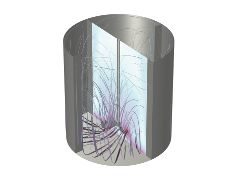
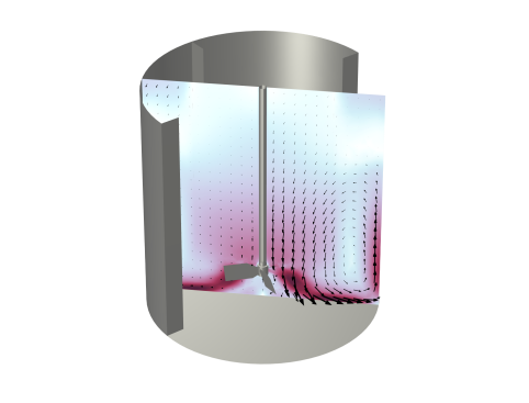
In the Settings window for 3D Plot Group, type Velocity Magnitude and Flow Direction in the Label text field.
3
Locate the Data section. From the Dataset list, choose Cut Plane 1.
4
From the Time (s) list, choose Last (4).
5
Locate the Title section. From the Title type list, choose None.
6
Locate the Plot Settings section. Clear the Plot dataset edges checkbox.
7
Locate the Color Legend section. Select the Show units checkbox.
Arrow Surface 1
1
Right-click Velocity Magnitude and Flow Direction and choose Arrow Surface.
2
In the Settings window for Arrow Surface, locate the Arrow Positioning section.
3
In the Number of arrows text field, type 500.
4
Locate the Coloring and Style section.
5
Select the Scale factor checkbox. In the associated text field, type 0.03.
6
From the Color list, choose Black.
Surface 1
1
In the Model Builder window, right-click Velocity Magnitude and Flow Direction and choose Surface.
2
In the Settings window for Surface, locate the Coloring and Style section.
3
From the Color table list, choose Passiflora.
Surface 2
Right-click Velocity Magnitude and Flow Direction and choose Surface.
Material Appearance 1
1
In the Model Builder window, right-click Surface 2 and choose Material Appearance.
2
In the Settings window for Material Appearance, locate the Appearance section.
3
From the Appearance list, choose Custom.
4
From the Material type list, choose Steel.
Surface 2
1
In the Model Builder window, click Surface 2.
2
In the Settings window for Surface, locate the Data section.
3
From the Dataset list, choose Study 2/Solution 2 (sol2).
Selection 1
1
Right-click Surface 2 and choose Selection.
2
In the Settings window for Selection, locate the Selection section.
3
From the Selection list, choose Union Selection 1.
4
In the list, choose 2, 11, and 12.
5
Click  Remove from Selection.
6
7
In the Velocity Magnitude and Flow Direction toolbar, click  Plot.
Create the plot in Figure 5. Start by creating Cut Line datasets for the different heights.
Cut Line 3D 1
1
In the Results toolbar, click  Cut Line 3D.
2
In the Settings window for Cut Line 3D, locate the Line Data section.
3
In row Point 1, set x to -0.005, y to T/2-0.12, and z to 0.458*H-C.
4
In row Point 2, set x to -0.005, y to T/2, and z to 0.458*H-C.
5
Locate the Data section. From the Dataset list, choose Study 2/Solution 2 (sol2).
6
Cut Line 3D 2
1
Right-click Cut Line 3D 1 and choose Duplicate.
2
In the Settings window for Cut Line 3D, locate the Line Data section.
3
In row Point 1, set z to 0.563*H-C.
4
In row Point 2, set z to 0.563*H-C.
Cut Line 3D 3
1
Right-click Cut Line 3D 2 and choose Duplicate.
2
In the Settings window for Cut Line 3D, locate the Line Data section.
3
In row Point 1, set z to 0.667*H-C.
4
In row Point 2, set z to 0.667*H-C.
Cut Line 3D 4
1
Right-click Cut Line 3D 3 and choose Duplicate.
2
In the Settings window for Cut Line 3D, locate the Line Data section.
3
In row Point 1, set z to 0.771*H-C.
4
In row Point 2, set z to 0.771*H-C.
Proceed to plot the axial velocity profiles.
Unscaled profiles
1
In the Results toolbar, click  1D Plot Group.
2
In the Settings window for 1D Plot Group, type Unscaled profiles in the Label text field.
3
Click to expand the Title section. From the Title type list, choose None.
4
Locate the Plot Settings section.
5
Select the x-axis label checkbox. In the associated text field, type y.
6
Select the y-axis label checkbox. In the associated text field, type U.
7
Locate the Axis section. Select the Manual axis limits checkbox.
8
In the x minimum text field, type 0.
9
In the x maximum text field, type 0.12.
10
Locate the Legend section. From the Position list, choose Upper left.
Line Graph 1
1
Right-click Unscaled profiles and choose Line Graph.
2
In the Settings window for Line Graph, locate the Data section.
3
From the Dataset list, choose Cut Line 3D 1.
4
From the Time selection list, choose Last.
5
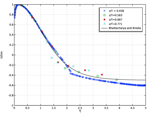
Locate the y-Axis Data section. In the Expression text field, type timeavg(3.5,4,idmap1(w),'nointerp'). This is the expression discussed in the Time averaging section.
6
Locate the x-Axis Data section. From the Parameter list, choose Expression.
7
In the Expression text field, type y.
8
Click to expand the Coloring and Style section. Find the Line markers subsection. From the Marker list, choose Diamond.
9
From the Positioning list, choose Interpolated.
10
In the Number text field, type 25.
11
Click to expand the Legends section. From the Legends list, choose Manual.
12
Select the Show legends checkbox.
13
Line Graph 2
1
Right-click Line Graph 1 and choose Duplicate.
2
In the Settings window for Line Graph, locate the Data section.
3
From the Dataset list, choose Cut Line 3D 2.
4
Locate the Coloring and Style section. Find the Line markers subsection. From the Marker list, choose Square.
5
Locate the Legends section. In the table, enter the following settings:
Line Graph 3
1
Right-click Line Graph 2 and choose Duplicate.
2
In the Settings window for Line Graph, locate the Data section.
3
From the Dataset list, choose Cut Line 3D 3.
4
Locate the Legends section. In the table, enter the following settings:
5
Locate the Coloring and Style section. Find the Line markers subsection. From the Marker list, choose Plus sign.
Line Graph 4
1
Right-click Line Graph 3 and choose Duplicate.
2
In the Settings window for Line Graph, locate the Data section.
3
From the Dataset list, choose Cut Line 3D 4.
4
Locate the Coloring and Style section. Find the Line markers subsection. From the Marker list, choose Triangle.
5
Locate the Legends section. In the table, enter the following settings:
6
In the Unscaled profiles toolbar, click  PlotIt takes some time to evaluate.
For the normalized axial velocity profile, determine the maximum velocity and the distance at which the velocity equals half of the maximum. With the help of Graph Markers, these values can be extracted from the results.
Graph Marker 1
1
In the Model Builder window, right-click Line Graph 1 and choose Graph Marker.
2
In the Settings window for Graph Marker, locate the Display section.
3
From the Display list, choose Max.
Add a Graph Marker to the remaining line graphs.
The values are displayed and saved to result tables. To evaluate the position of half the maximum velocity, the value for the respective maximum velocity is needed.
Parameters
1
In the Model Builder window, expand the Results > Tables node.
2
Right-click Results and choose Parameters.
For convenience, these parameters along with additional ones to be used later, are available in a file.
3
In the Settings window for Parameters, locate the Parameters section.
4
Click  Load from File.
5
Add new Graph Markers using the Ymax values.
Graph Marker 2
1
In the Model Builder window, right-click Line Graph 1 and choose Graph Marker.
2
In the Settings window for Graph Marker, locate the Display section.
3
From the Display mode list, choose Line intersection.
4
From the Line type list, choose Horizontal.
5
In the y-coordinates text field, type Ymax1/2.
Repeat for the remaining line graphs.
Line Graph 2
1
In the Model Builder window, under Results > Unscaled profiles click Line Graph 2.
2
In the Unscaled profiles toolbar, click  Plot.
The values of the intersections are again stored in their respective tables. The first value corresponds to the Xhalf values in the Parameters list.
With this, the normalized profile can be plotted. First, write the data for each graph into a table.
Line Graph 1
1
In the Model Builder window, right-click Line Graph 1 and choose Copy Plot Data to Table.
Repeat for the remaining line graphs.
Now, the tables can be used to create Figure 5 by scaling them using the parameters evaluated before.
Scaled profiles
1
In the Results toolbar, click  1D Plot Group.
2
In the Settings window for 1D Plot Group, type Scaled profiles in the Label text field.
3
Locate the Title section. From the Title type list, choose None.
4
Locate the Plot Settings section.
5
Select the x-axis label checkbox. In the associated text field, type \eta.
6
Select the y-axis label checkbox. In the associated text field, type U/Um.
7
Locate the Axis section. Select the Manual axis limits checkbox.
8
In the x minimum text field, type 0.
9
In the x maximum text field, type 5.
Leave the y-axis limits at their default values.
Table Graph 1
1
Right-click Scaled profiles and choose Table Graph.
2
In the Settings window for Table Graph, locate the Data section.
3
From the Table list, choose Table 1.
4
Click to expand the Preprocessing section. Find the x-axis column subsection. From the Transformation list, choose Linear.
5
In the Scaling text field, type -scaleX1.
6
In the Shift text field, type T/2*scaleX1.
7
Find the y-axis columns subsection. From the Transformation list, choose Linear.
8
In the Scaling text field, type 1/Ymax1.
9
Locate the Coloring and Style section. Find the Line style subsection. From the Line list, choose None.
10
Find the Line markers subsection. From the Marker list, choose Diamond.
11
Click to expand the Legends section. From the Legends list, choose Manual.
12
Select the Show legends checkbox.
13
Table Graph 2
1
Right-click Table Graph 1 and choose Duplicate.
2
In the Settings window for Table Graph, locate the Data section.
3
From the Table list, choose Table 2.
4
Locate the Preprocessing section. Find the x-axis column subsection. In the Scaling text field, type -scaleX2.
5
In the Shift text field, type T/2*scaleX2.
6
Find the y-axis columns subsection. In the Scaling text field, type 1/Ymax2.
7
Locate the Coloring and Style section. Find the Line markers subsection. From the Marker list, choose Square.
8
From the Positioning list, choose Interpolated.
9
Locate the Legends section. In the table, enter the following settings:
Table Graph 3
1
Right-click Table Graph 2 and choose Duplicate.
2
In the Settings window for Table Graph, locate the Data section.
3
From the Table list, choose Table 3.
4
Locate the Preprocessing section. Find the x-axis column subsection. In the Scaling text field, type -scaleX3.
5
In the Shift text field, type T/2*scaleX3.
6
Find the y-axis columns subsection. In the Scaling text field, type 1/Ymax3.
7
Locate the Coloring and Style section. Find the Line markers subsection. From the Marker list, choose Plus sign.
8
Locate the Legends section. In the table, enter the following settings:
Table Graph 4
1
Right-click Table Graph 3 and choose Duplicate.
2
In the Settings window for Table Graph, locate the Data section.
3
From the Table list, choose Table 4.
4
Locate the Preprocessing section. Find the x-axis column subsection. In the Scaling text field, type -scaleX4.
5
In the Shift text field, type T/2*scaleX4.
6
Find the y-axis columns subsection. In the Scaling text field, type 1/Ymax4.
7
Locate the Coloring and Style section. Find the Line markers subsection. From the Marker list, choose Triangle.
8
Locate the Legends section. In the table, enter the following settings:
Scaled profiles
Finally, add the plot for Equation 2.
Line Graph 1
1
In the Model Builder window, right-click Scaled profiles and choose Line Graph.
2
In the Settings window for Line Graph, locate the Data section.
3
From the Dataset list, choose Cut Line 3D 1.
4
From the Time selection list, choose Last.
5
Locate the y-Axis Data section. In the Expression text field, type 1-1.5*tanh(0.78*(y*50-0.15))^2.
6
Locate the x-Axis Data section. From the Parameter list, choose Expression.
7
In the Expression text field, type y*50.
8
Locate the Coloring and Style section. From the Color list, choose Black.
9
Locate the Legends section. From the Legends list, choose Manual.
10
Select the Show legends checkbox.
11
Scaled profiles
1
In the Model Builder window, click Scaled profiles.
2
In the Scaled profiles toolbar, click  Plot.