
|
|
|
|
1
|
|
2
|
In the Select Physics tree, select Fluid Flow > Multiphase Flow > Rotating Machinery, Phase Transport Mixture Model > Turbulent Flow > Turbulent Flow, k-ε.
|
|
3
|
Click Add.
|
|
4
|
Click
|
|
5
|
|
6
|
Click
|
|
1
|
|
2
|
|
3
|
Click
|
|
4
|
Browse to the model’s Application Libraries folder and double-click the file three_phase_mixer.mphbin.
|
|
1
|
|
2
|
|
3
|
|
4
|
|
1
|
|
2
|
|
3
|
|
4
|
Select the Cutoff checkbox.
|
|
5
|
|
1
|
|
2
|
Go to the Add Material window.
|
|
3
|
|
4
|
Click the Add to Component button in the window toolbar.
|
|
5
|
|
2
|
|
3
|
|
1
|
|
2
|
|
3
|
Select the Include gravity checkbox.
|
|
1
|
|
3
|
|
4
|
|
1
|
|
1
|
|
2
|
|
3
|
Click
|
|
1
|
In the Model Builder window, under Component 1 (comp1) > Phase Transport (phtr) click Initial Values 1.
|
|
2
|
|
3
|
|
4
|
|
1
|
In the Model Builder window, under Component 1 (comp1) > Multiphysics click Mixture Model 1 (mfmm1).
|
|
2
|
|
3
|
From the Mixture viscosity model list, choose User defined. In the μ text field, type mfmm1.muc*max(1-max(0,min(s2+s3,0.999*0.62))/0.62,eps)^(-2.5*0.62).
|
|
4
|
|
5
|
Locate the Dispersed Phase 2 Properties section. From the ρs2 list, choose User defined. In the associated text field, type 1100[kg/m^3].
|
|
6
|
Locate the Dispersed Phase 3 Properties section. From the ρs3 list, choose User defined. In the associated text field, type 850[kg/m^3].
|
|
1
|
|
2
|
|
3
|
|
4
|
|
5
|
|
1
|
In the Model Builder window, expand the Component 1 (comp1) > Mesh 1 > Boundary Layers 1 node, then click Boundary Layer Properties 1.
|
|
2
|
|
3
|
|
4
|
|
1
|
|
2
|
|
3
|
|
1
|
|
2
|
|
3
|
In the Model Builder window, under Study 1 > Solver Configurations > Solution 1 (sol1) click Time-Dependent Solver 1.
|
|
4
|
|
5
|
|
6
|
Find the Algebraic variable settings subsection. In the Fraction of initial step for Backward Euler text field, type 1.
|
|
7
|
In the Model Builder window, expand the Study 1 > Solver Configurations > Solution 1 (sol1) > Time-Dependent Solver 1 > Segregated 1 node, then click Velocity u, Pressure p.
|
|
8
|
|
9
|
|
10
|
In the Model Builder window, under Study 1 > Solver Configurations > Solution 1 (sol1) > Time-Dependent Solver 1 > Segregated 1 click Volume Fractions.
|
|
11
|
|
12
|
|
13
|
|
14
|
Click
|
|
1
|
|
2
|
|
3
|
|
4
|
|
5
|
|
6
|
|
1
|
|
2
|
|
3
|
|
4
|
|
5
|
|
6
|
|
1
|
|
2
|
|
3
|
Click
|
|
4
|
|
5
|
Click OK.
|
|
1
|
|
2
|
|
3
|
|
4
|
|
1
|
|
2
|
|
3
|
|
4
|
|
1
|
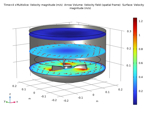
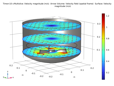
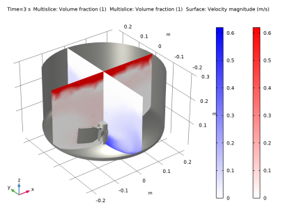
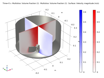
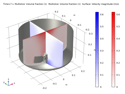
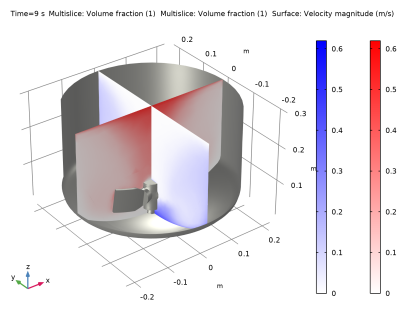
In the Model Builder window, expand the Results > Volume Fraction (phtr) node, then click Volume Fraction (phtr).
|
|
2
|
|
3
|
|
1
|
|
2
|
|
3
|
|
4
|
|
5
|
|
6
|
|
7
|
|
8
|
|
9
|
|
10
|
|
11
|
|
1
|
|
2
|
|
3
|
|
4
|
|
5
|
|
6
|
|
1
|
|
2
|
Clear the Plot dataset edges checkbox.
|
|
3
|
|
4
|
|
1
|
|
2
|
|
3
|
|
1
|
|
2
|
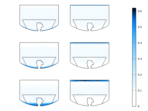
In the Settings window for 2D Plot Group, type Volume Fraction at Different Times in the Label text field.
|
|
1
|
|
2
|
|
3
|
|
4
|
|
5
|
|
6
|
|
7
|
|
1
|
|
2
|
|
3
|
|
4
|
|
5
|
|
1
|
In the Model Builder window, under Results > Volume Fraction at Different Times right-click Surface 1 and choose Duplicate.
|
|
2
|
|
3
|
|
4
|
|
5
|
|
1
|
|
2
|
|
3
|
|
1
|
In the Model Builder window, under Results > Volume Fraction at Different Times right-click Surface 1 and choose Duplicate.
|
|
2
|
|
3
|
|
4
|
|
1
|
|
2
|
|
3
|
|
4
|
|
1
|
|
2
|
|
3
|
|
1
|
|
2
|
|
3
|
|
4
|
|
5
|