|
|
|



|
1
|
|
2
|
In the Select Physics tree, select Fluid Flow > Single-Phase Flow > Rotating Machinery, Fluid Flow > Turbulent Flow > Turbulent Flow, k-ε.
|
|
3
|
Click Add.
|
|
4
|
Click
 Study. Study. |
|
5
|
In the Select Study tree, select Preset Studies for Selected Physics Interfaces > Frozen Rotor with Stationary Free Surface.
|
|
6
|
Click
 Done. Done. |
|
1
|
|
2
|
Browse to the model’s Application Libraries folder and double-click the file free_surface_mixer_geom_sequence.mph.
|
|
3
|
|
4
|
|
1
|
|
2
|
|
1
|
|
2
|
|
3
|
|
4
|
|
5
|
Click
 Plot. Plot. |
|
1
|
|
3
|
|
4
|
|
5
|
|
1
|
|
1
|
|
2
|
|
3
|
Select the Include gravity checkbox.
|
|
1
|
|
3
|
|
4
|
|
1
|
|
2
|
|
3
|
|
1
|
|
2
|
|
3
|
|
1
|
|
2
|
Go to the Add Material window.
|
|
3
|
|
4
|
Right-click and choose Add to Component 1 (comp1).
|
|
5
|
|
1
|
|
1
|
|
2
|
|
3
|
|
4
|
|
1
|
|
2
|
|
3
|
Click the Custom button.
|
|
4
|
|
5
|
|
6
|
|
1
|
|
2
|
|
3
|
|
4
|
Click the Custom button.
|
|
5
|
Locate the Element Size Parameters section.
|
|
6
|
|
7
|
|
8
|
|
9
|
Select the Curvature factor checkbox.
|
|
10
|
Select the Resolution of narrow regions checkbox.
|
|
1
|
|
2
|
|
3
|
|
5
|
Click the
 Wireframe Rendering button in the Graphics toolbar to be able to locate the entities inside the vessel. Wireframe Rendering button in the Graphics toolbar to be able to locate the entities inside the vessel. |
|
1
|
|
2
|
|
3
|
|
4
|
Click
 Paste Selection. Paste Selection. |
|
5
|
|
6
|
Click OK.
|
|
7
|
|
8
|
|
9
|
Click the Custom button.
|
|
10
|
Locate the Element Size Parameters section.
|
|
11
|
|
12
|
|
1
|
|
2
|
|
3
|
|
4
|
Click
 Paste Selection. Paste Selection. |
|
5
|
|
6
|
Click OK.
|
|
7
|
|
8
|
|
1
|
|
2
|
|
3
|
|
1
|
|
2
|
|
3
|
|
4
|
|
5
|
|
1
|
|
2
|
|
3
|
|
4
|
|
5
|
|
1
|
In the Model Builder window, expand the Boundary Layers 1 node, then click Boundary Layer Properties 1.
|
|
2
|
|
3
|
|
4
|
|
5
|
Click
 Build All. Build All. |
|
6
|
|
1
|
|
2
|
|
3
|
|
1
|
|
2
|
|
3
|
|
1
|
|
2
|
|
3
|
|
1
|
|
2
|
|
3
|
|
4
|
Click
 Build All. Build All. |
|
1
|
|
2
|
|
3
|
|
1
|
|
2
|
|
3
|
|
1
|
|
2
|
|
1
|
|
2
|
|
3
|
|
4
|
Click
 Build All. Build All. |
|
1
|
|
2
|
|
3
|
Select the Modify model configuration for study step checkbox.
|
|
4
|
|
5
|
Click
 Disable. Disable. |
|
6
|
Click to expand the Mesh Selection section. In the table, enter the following settings:
|
|
7
|
|
8
|
Click
 Add. Add. |
|
10
|
|
11
|
|
12
|
|
13
|
In the Show More Options dialog, in the tree, select the checkbox for the node Study > Multigrid Level.
|
|
14
|
Click OK.
|
|
15
|
|
16
|
|
18
|
|
1
|
In the Settings window for Stationary Free Surface, locate the Physics and Variables Selection section.
|
|
2
|
Select the Modify model configuration for study step checkbox.
|
|
3
|
|
4
|
Right-click and choose Disable.
|
|
5
|
Click to expand the Mesh Selection section. In the table, enter the following settings:
|
|
1
|
|
2
|
|
3
|
In the Model Builder window, expand the Study 1 > Solver Configurations > Solution 1 (sol1) > Stationary Solver 1 > Segregated 1 node.
|
|
4
|
In the Model Builder window, expand the Study 1 > Solver Configurations > Solution 1 (sol1) > Stationary Solver 1 > AMG, fluid flow variables (spf_spatial1) node, then click Multigrid 1.
|
|
5
|
|
6
|
|
7
|
|
1
|
|
2
|
|
3
|
Select the Only plot when requested checkbox.
|
|
4
|
|
5
|
|
6
|
Clear the Plot dataset edges checkbox.
|
|
1
|
|
2
|
|
1
|
|
2
|
|
3
|
|
1
|
|
2
|
|
3
|
|
1
|
|
2
|
|
3
|
|
4
|
|
5
|
|
6
|
|
1
|
|
2
|
|
3
|
|
4
|
|
5
|
|
6
|
Locate the Coloring and Style section.
|
|
7
|
|
1
|
|
2
|
|
3
|
|
1
|
|
2
|
|
3
|
|
4
|
|
5
|
|
1
|
|
2
|
|
3
|
|
4
|
|
5
|
Click
 Remove from Selection. Remove from Selection. |
|
7
|
|
1
|
|
2
|
|
3
|
|
1
|
|
2
|
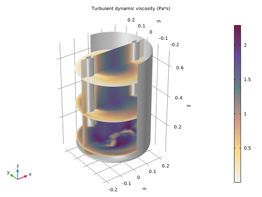
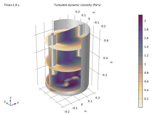
In the Settings window for Multislice, click Replace Expression in the upper-right corner of the Expression section. From the menu, choose Component 1 (comp1) > Turbulent Flow, k-ε > Turbulence variables > spf.muT - Turbulent dynamic viscosity - Pa·s.
|
|
3
|
|
4
|
|
5
|
|
1
|
|
2
|
|
3
|
|
4
|
|
5
|
|
1
|
|
2
|
|
3
|
|
4
|
|
5
|
Click
 Remove from Selection. Remove from Selection. |
|
7
|
|
1
|
|
2
|
|
3
|
|
1
|
|
2
|
|
3
|
|
4
|
|
1
|
|
2
|
Go to the Add Study window.
|
|
3
|
|
4
|
Right-click and choose Add Study.
|
|
5
|
|
1
|
|
2
|
|
3
|
Click to expand the Values of Dependent Variables section. Find the Initial values of variables solved for subsection. From the Settings list, choose User controlled.
|
|
4
|
|
5
|
|
6
|
|
7
|
Click to expand the Mesh Selection section. In the table, enter the following settings:
|
|
8
|
|
9
|
|
10
|
Clear the Generate default plots checkbox because you can duplicate the previous plots and only need top update the dataset.
|
|
11
|
|
1
|
In the Model Builder window, under Results, Ctrl-click to select Velocity (spf), Pressure (spf), Wall Resolution (spf), Turbulent Viscosity, and Velocity xy.
|
|
2
|
Right-click and choose Group.
|
|
1
|
|
2
|
|
1
|
|
2
|
|
3
|
|
4
|
|
1
|
In the Model Builder window, expand the Results > Time Dependent > Velocity (spf) 1 > Surface 1 node.
|
|
2
|
|
1
|
|
2
|
|
3
|
Select the Plot checkbox.
|
|
1
|
|
2
|
|
3
|
|
4
|
|
5
|
|
1
|
|
2
|
|
3
|
|
1
|
|
2
|
|
3
|
|
4
|
|
1
|
|
2
|
|
3
|
|
4
|
|
1
|
|
2
|
|
3
|
|
1
|
|
2
|
|
3
|
|
4
|
|
5
|
Locate the Coloring and Style section.
|
|
6
|
|
7
|