|
|
|


|
1
|
|
2
|
|
3
|
Click Add.
|
|
4
|
|
5
|
Click Add.
|
|
6
|
Click
|
|
7
|
|
8
|
Click
|
|
1
|
|
2
|
|
3
|
|
1
|
|
2
|
|
1
|
|
2
|
|
3
|
|
4
|
|
5
|
Click
|
|
1
|
|
2
|
|
3
|
|
4
|
|
5
|
|
6
|
|
7
|
Click
|
|
1
|
|
2
|
Select the object r1 only.
|
|
3
|
|
4
|
|
5
|
Select the object r2 only.
|
|
6
|
Click
|
|
1
|
|
2
|
On the object dif1, select Points 3 and 5 only.
|
|
3
|
|
4
|
|
5
|
Click
|
|
1
|
|
2
|
On the object fil1, select Points 1 and 9 only.
|
|
3
|
|
4
|
|
5
|
Click
|
|
1
|
|
2
|
Select the object fil2 only.
|
|
3
|
|
4
|
Select the Keep input objects checkbox.
|
|
5
|
|
6
|
|
7
|
Click
|
|
1
|
|
2
|
Click in the Graphics window and then press Ctrl+A to select both objects.
|
|
3
|
|
1
|
In the Model Builder window, under Component 1 (comp1) > Geometry 1 right-click Work Plane 1 (wp1) and choose Extrude.
|
|
2
|
|
4
|
Click
|
|
5
|
|
1
|
|
2
|
|
0.5 m6/mol²
|
|
1
|
In the Model Builder window, under Component 1 (comp1) right-click Materials and choose Blank Material.
|
|
2
|
|
1
|
|
3
|
|
4
|
From the list, choose Fully developed flow.
|
|
5
|
|
6
|
|
1
|
|
1
|
|
1
|
|
2
|
In the Settings window for Transport of Diluted Species, click to expand the Discretization section.
|
|
3
|
|
1
|
In the Model Builder window, under Component 1 (comp1) > Transport of Diluted Species (tds) click Fluid 1.
|
|
2
|
|
3
|
|
1
|
|
3
|
|
4
|
Select the Species c checkbox.
|
|
5
|
|
1
|
|
3
|
|
4
|
Select the Species c checkbox.
|
|
1
|
|
2
|
|
3
|
Click
|
|
4
|
|
5
|
Click OK.
|
|
1
|
|
2
|
|
3
|
Click
|
|
4
|
|
5
|
Click OK.
|
|
1
|
|
2
|
|
3
|
|
4
|
|
1
|
|
2
|
|
3
|
Click
|
|
4
|
|
5
|
Click OK.
|
|
1
|
In the Model Builder window, expand the Component 1 (comp1) > Mesh 1 > Boundary Layers 1 node, then click Boundary Layer Properties 1.
|
|
2
|
|
3
|
Click
|
|
4
|
|
5
|
Click OK.
|
|
6
|
|
1
|
|
2
|
|
3
|
Clear the Generate default plots checkbox.
|
|
1
|
|
2
|
|
3
|
In the Solve for column of the table, under Component 1 (comp1), clear the checkbox for Transport of Diluted Species (tds).
|
|
1
|
|
2
|
|
3
|
In the Solve for column of the table, under Component 1 (comp1), clear the checkbox for Creeping Flow (spf).
|
|
4
|
|
5
|
Click
|
|
7
|
|
1
|
|
2
|
|
3
|
|
4
|
Click
|
|
5
|
In the Paste Selection dialog, type 1 3 5 6 7 8 11 12 13 14 15 17 18 19 20 21 22 24 26 27 in the Selection text field.
|
|
6
|
Click OK.
|
|
1
|
|
2
|
|
1
|
|
2
|
|
3
|
|
1
|
|
2
|
|
3
|
|
4
|
|
5
|
|
6
|
|
7
|
|
1
|
|
2
|
|
3
|
|
4
|
|
1
|
|
2
|
|
3
|
|
4
|
|
5
|
|
6
|
|
7
|
|
1
|
|
2
|
|
3
|
|
1
|
|
2
|
|
3
|
|
4
|
|
5
|
|
1
|
|
2
|
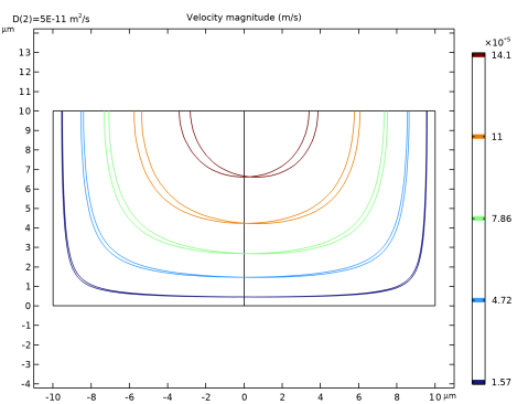
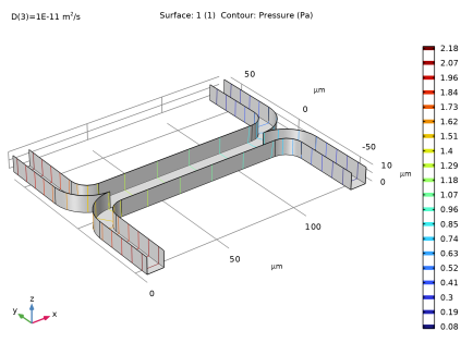
In the Settings window for Contour, click Replace Expression in the upper-right corner of the Expression section. From the menu, choose Component 1 (comp1) > Creeping Flow > Velocity and pressure > p - Pressure - Pa.
|
|
3
|
|
1
|
|
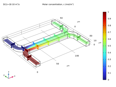
2
|
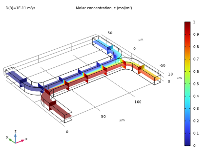
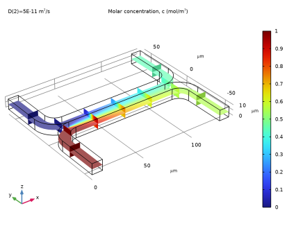
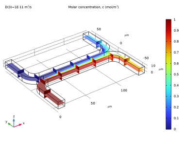
In the Settings window for 3D Plot Group, type Concentration (Uncoupled Flow) in the Label text field.
|
|
1
|
|
2
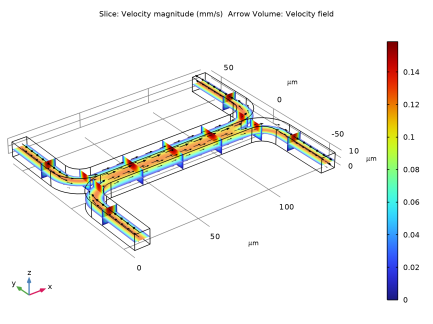
|
In the Settings window for Slice, click Replace Expression in the upper-right corner of the Expression section. From the menu, choose Component 1 (comp1) > Transport of Diluted Species > Species c > c - Molar concentration, c - mol/m³.
|
|
1
|
|
2
|
In the Settings window for Slice, click Replace Expression in the upper-right corner of the Expression section. From the menu, choose c - Molar concentration, c - mol/m³.
|
|
1
|
|
2
|
In the Settings window for Slice, click Replace Expression in the upper-right corner of the Expression section. From the menu, choose c - Molar concentration, c - mol/m³.
|
|
1
|
|
2
|
|
3
|
|
4
|
|
1
|
|
2
|
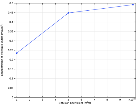
In the Settings window for 1D Plot Group, type Output Concentration (Uncoupled Flow) in the Label text field.
|
|
1
|
|
2
|
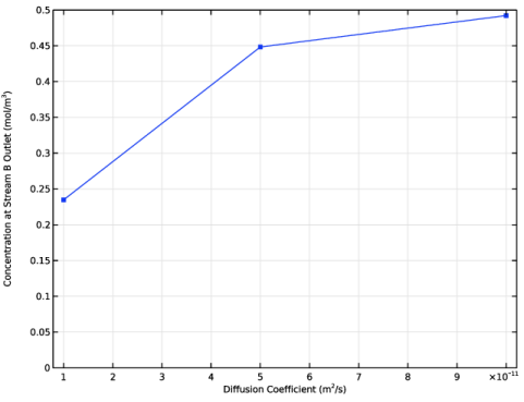
In the Settings window for Global, click Replace Expression in the upper-right corner of the y-Axis Data section. From the menu, choose Component 1 (comp1) > Transport of Diluted Species > Outflow 2 > tds.out2.c0_avg_c - Average concentration - mol/m³.
|
|
3
|
|
4
|
Click to expand the Coloring and Style section. Find the Line markers subsection. From the Marker list, choose Point.
|
|
5
|
|
6
|
|
1
|
|
2
|
|
3
|
|
4
|
Locate the Plot Settings section.
|
|
5
|
Select the x-axis label checkbox. In the associated text field, type Diffusion Coefficient (m<sup>2</sup>/s).
|
|
6
|
Select the y-axis label checkbox. In the associated text field, type Concentration at Stream B Outlet (mol/m<sup>3</sup>).
|
|
7
|
|
8
|
|
9
|
|
10
|
|
1
|
In the Model Builder window, under Component 1 (comp1) > Creeping Flow (spf) click Fluid Properties 1.
|
|
2
|
In the Settings window for Fluid Properties, type Fluid Properties: Uncoupled in the Label text field.
|
|
1
|
|
2
|
In the Settings window for Fluid Properties, type Fluid Properties: Coupled in the Label text field.
|
|
3
|
Locate the Fluid Properties section. From the μ list, choose User defined. In the associated text field, type 1e-3[Pa*s]*(1+alpha*c^2).
|
|
1
|
|
2
|
|
3
|
Select the Modify model configuration for study step checkbox.
|
|
4
|
|
5
|
Right-click and choose Disable.
|
|
1
|
|
2
|
Go to the Add Study window.
|
|
3
|
|
4
|
Click the Add Study button in the window toolbar.
|
|
5
|
|
1
|
|
2
|
Clear the Generate default plots checkbox.
|
|
3
|
|
1
|
|
2
|
|
3
|
|
1
|
|
2
|
|
3
|
|
4
|
|
1
|
|
2
|
|
3
|
|
4
|
|
1
|
|
2
|
In the Settings window for 3D Plot Group, type Concentration (Coupled Flow) in the Label text field.
|
|
3
|
|
4
|
|
1
|
|
2
|
|
3
|
|
1
|
|
2
|
|
3
|
|
1
|
|
2
|
|
3
|
|
4
|
|
1
|
|
2
|
|
3
|
|
1
|
|
2
|
|
3
|
|
4
|
|
5
|
|
6
|
|
7
|
|
8
|
|
1
|
|
2
|
In the Settings window for Global Evaluation, click Replace Expression in the upper-right corner of the Expressions section. From the menu, choose Component 1 (comp1) > Transport of Diluted Species > Outflow 2 > tds.out2.c0_avg_c - Average concentration - mol/m³.
|
|
3
|
Click
|
|
1
|
|
2
|
|
3
|
|
4
|