PDF

Quenching of a Steel Billet
Introduction
Quenching is a heat treating process that is used to tailor the microstructure, and to control distortions and residual stresses in steel components. If distortions can be minimized, postquenching manufacturing operations such as grinding can be avoided. From an endurance standpoint, compressive residual stresses at the surface of a component can be beneficial because the propensity for fatigue failure is reduced. A tendency is to try to use steel components as heat treated. This preserves beneficial compressive stresses on the surface, and reduces overall manufacturing costs.
In this example, a steel billet is considered. The billet is first heated to 900°C, and then quenched in oil. As the temperature decreases, the austenite decomposes into a combination of ferrite, pearlite, bainite, and martensite. The model shows how to define the temperature-dependent metallurgical phase transformations that are involved in this process, and how to compute the heterogeneous phase composition in the billet. During quenching, phase transformation strains produce stresses and deformations. The model shows how to compute these stresses and deformations by coupling the temperature-dependent phase transformations to an elastoplastic analysis. Effects such as traditional plasticity as well as transformation induced plasticity (TRIP) are included.
Model Definition
The steel billet is a solid cylinder that is 20 cm in length and with a radius of 2 cm. The billet is quenched in oil, uniformly across its boundary, through a temperature-dependent heat transfer coefficient. Because of symmetries, only half the billet is considered, in 2D axisymmetry. The billet is shown in Figure 1. Thermal and mechanical boundary conditions are discussed below.
Material Properties
The material properties of the steel billet are temperature-dependent, and also phase dependent. The Austenite Decomposition physics interface automatically averages these properties into effective properties that define a compound material. The compound material is used in the thermal and mechanical analyses.
Figure 1: The axisymmetric model of the steel billet.
Phase Transformation Analysis
During cooling, the austenite can decompose into a combination of ferrite, pearlite, bainite, and martensite. The phase transformation into martensite is displacive and described by the Koistinen–Marburger model. The model states that the amount of martensite formed at the expense of austenite depends on the fraction of available austenite, and under-cooling below the so-called martensite start temperature Ms. On differential form, the model is given by
where the rate at which the destination phase (martensite) forms is proportional to the temperature rate and the instantaneous fraction of the source phase (austenite), through the Koistinen–Marburger coefficient β. Note that martensite only forms during cooling, meaning that the temperature rate must be negative. The remaining diffusive phase transformations are modeled using the Leblond–Devaux model. This model is characterized by a contributing term that is proportional to the available fraction of the source phase, and a retardation term that is proportional to the current fraction of formed destination phase. The proportionality is given by two temperature-dependent functions K and L.
The parameters that are required to describe the austenite decomposition into ferrite, pearlite, and bainite are given in Table 1, Table 2, and Table 3 below.
K (1/s)
L (1/s)
K (1/s)
L (1/s)
K (1/s)
L (1/s)
Martensite forms at the expense of the available fraction of source phase (austenite), and the two parameters that define this phase transformation are given in Table 4.
Ms
300°C
β
Thermal Analysis
The heat transport in the bar is described by the heat equation:
where T is the temperature, k represents the thermal conductivity, ρ denotes the density, Cp denotes the specific heat capacity, and Q is a heat source. The thermal conductivity, the density, and the specific heat capacity are in general temperature dependent, but in the presence of metallurgical phase transformations, they also depend on the current phase composition. For example, the thermal conductivity of austenite is different from that of ferrite, and as the phase fractions evolve, so will the thermal conductivity of the compound material. In the present thermal analysis, phase transformation latent heat is neglected so that Q = 0. The densities, specific heat capacities and heat conductivities of the individual metallurgical phases are given in Table 5.
ρ (kg/m3)
 Cp (J/(kg·K))
k (W/(m·K))
In the model, it is assumed that ferrite, pearlite, and bainite share thermal properties. Furthermore, from a thermal diffusivity standpoint, it is assumed that the densities of the individual phases are temperature independent.
Boundary Conditions
The quenching oil is not modeled explicitly, but it is replaced by a temperature-dependent heat transfer coefficient h that is used to prescribe a heat flux as
where Text = 80°C is the temperature of the quenching oil. The heat transfer properties of the quenching oil are shown in Table 6.
h (W/(m2·K))
Mechanical Analysis
The quenching process is time dependent, but from a structural-mechanics point of view it is quasi static, and modeled as such. Stresses and strains are computed using material properties of the compound material defined by the phase composition and the constitutive behavior of the individual phases.
Material Properties
As in thermal analysis, the mechanical analysis involves material properties that are temperature as well as phase composition dependent. In this model, the elastoplastic behavior of the individual metallurgical phases is taken to be linear elastic with linear hardening. The mechanical material properties are shown in Table 7. The linear elastic behavior is given by the Young’s moduli (E) and Poisson’s ratios (ν) of the phases, and the plastic behavior is given by initial yield stresses (σys0) and isotropic hardening moduli (h). In this model, the elastic behavior is assumed to be equal between phases. Note that the secant coefficients of thermal expansion (α) are not averaged into a compound material property, but are instead used to compute the thermal strain tensor of each metallurgical phase. The thermal strain tensors are averaged into a thermal strain of the compound material.
E (GPa)
ν
σys0 (MPa)
h (GPa)
  α (1/K)
To complete the description of the phase properties, a volume reference temperature Tref has to be defined for each metallurgical phase. The choice of volume reference temperature is to an extent arbitrary. In this model, the heating stage (austenitization) is not considered explicitly, so the volume reference temperature is set to the austenitization temperature (900°C). This means that the billet is strain free at this temperature. To account for the strains that follow from thermal expansion and austenitization of the (unknown) base phase composition, an initial strain is applied.
Boundary Conditions
Only half the billet is modeled, and a displacement symmetry boundary condition is applied to the midplane.
Transformation Induced Plasticity (TRIP)
In general, phase transformations occur while the material is subjected to a mechanical stress. This gives rise to so-called transformation induced plasticity, or TRIP. In essence, an inelastic straining of the material results from stresses that are below the yield stress, and would not cause plastic flow in a classical plasticity sense. In this model, the TRIP effect is included in each phase transformation. Two parameters are required to describe the effect: the parameter and the saturation function Φ. For simplicity, and with no additional experimental support, both are used with their default values for every phase transformation in the model.
Phase Plasticity
It is possible to allow for plasticity in the individual phases. By default, the equivalent plastic strain of the individual phases follows that of the compound material. That is to say, the equivalent plastic strain of a given phase in the Austenite Decomposition interface is equal to the equivalent plastic strain of a Plasticity node under Solid Mechanics. This equivalence is established through the Phase Transformation Strain multiphysics coupling. For the vanishing austenite, this is a reasonable modeling assumption. However, for phases that appear gradually and devoid of prior plastic straining, this assumption is questionable. Following Ref. 1, this deficiency can be remedied by allowing for plastic recovery of the destination phase. This is done for every destination phase in the model.
Initial Strains from Heating and Austenitization
To account for the strains that follow from thermal expansion and austenitization of the (unknown) base phase composition, an initial strain is applied. The initial strain is given by
Results and Discussion
When the billet is cooled, the austenite decomposes into a combination of ferrite, pearlite, bainite, and martensite. Because of the inhomogeneous rate of cooling, the resulting phase composition will differ throughout the billet. For example, the ends of the billet experience a higher rate of cooling than the mid section. This suggests that the ferritic, pearlitic, and bainitc phase transformations are reduced in favor of the transformation to martensite, as this transformation is controlled by the amount of undercooling beneath the start temperature Ms, see Figure 2 (left).
During cooling, the material in the billet undergoes straining. Thermal strains result from the change in temperature, and mechanical stresses cause transformation induced plasticity (TRIP). Stresses exceed the initial yield stress of the compound material. This can be seen in Figure 2 (middle), where the largest equivalent plastic strain is observed on the surface of the billet. The quenching simulation computes residual stresses. In Figure 2 (right), the axial stress is shown. Note that the stresses are compressive on the surface of the billet. This is usually beneficial from a fatigue standpoint.
Figure 2: Phase fraction of martensite (left), equivalent plastic strain (middle), and axial tensile stress (right).
The evolving phase composition is shown for two locations at the mid plane of the billet: Figure 3 shows the phase composition on the surface, and Figure 4 the phase composition at the billet center. Comparing these phase compositions, the final fraction of martensite is higher at the surface than at the center of the billet. At the surface, the cooling rate is governed by the heat transfer coefficient and the temperature difference between the surface and the quenching oil. If the oil is able to provide a high enough rate of cooling, diffusion controlled phase transformations are limited in favor of the displacive martensitic transformation. In contrast, the cooling rate of a material point at the center of the billet is limited by the thermal diffusivity of the material. It is common to add certain alloying elements to the material to alter the phase transformation characteristics. This way certain diffusion-controlled phase transformations can be reduced or even suppressed.
Figure 3: Phase composition on the surface of the steel billet middle.
Figure 4: Phase composition at the billet center.
References
1. J.B. Leblond, “Mathematical modelling of transformation plasticity in steels II: Coupling with strain hardening phenomena,” Int. J. Plast., vol. 5, pp. 573–591, 1989.
Application Library path: Metal_Processing_Module/Steel_Quenching/quenching_of_a_steel_billet
Modeling Instructions
From the File menu, choose New.
New
In the New window, click  Model Wizard.
Model Wizard
1
In the Model Wizard window, click  2D Axisymmetric.
2
In the Select Physics tree, select Heat Transfer > Metal Processing > Steel Quenching.
3
Click Add.
4
Click  Study.
5
In the Select Study tree, select General Studies > Time Dependent.
6
Geometry 1
Create a node group that contains the temperature dependent data for the transformation of austenite to ferrite.
Global Definitions
Austenite to Ferrite
1
In the Model Builder window, right-click Global Definitions and choose Node Group.
2
In the Settings window for Group, type Austenite to Ferrite in the Label text field.
Interpolation 1 (int1)
1
In the Home toolbar, click  Functions and choose Global > Interpolation.
2
In the Settings window for Interpolation, locate the Definition section.
3
In the Function name text field, type K_Austenite_to_Ferrite.
4
Click  Load from File.
5
Browse to the model’s Application Libraries folder and double-click the file quenching_of_a_steel_billet_K_Austenite_to_Ferrite.txt.
6
Locate the Interpolation and Extrapolation section. From the Interpolation list, choose Piecewise cubic.
7
Locate the Units section. In the Argument table, enter the following settings:
8
In the Function table, enter the following settings:
Interpolation 2 (int2)
1
In the Home toolbar, click  Functions and choose Global > Interpolation.
2
In the Settings window for Interpolation, locate the Definition section.
3
In the Function name text field, type L_Austenite_to_Ferrite.
4
Click  Load from File.
5
Browse to the model’s Application Libraries folder and double-click the file quenching_of_a_steel_billet_L_Austenite_to_Ferrite.txt.
6
Locate the Interpolation and Extrapolation section. From the Interpolation list, choose Piecewise cubic.
7
Locate the Units section. In the Argument table, enter the following settings:
8
In the Function table, enter the following settings:
Create node groups and interpolation functions in a similar fashion for the austenite transformation into pearlite and bainite. Load the appropriate functions from file.
Read temperature dependent data for the Young’s modulus.
Interpolation 7 (int7)
1
In the Home toolbar, click  Functions and choose Global > Interpolation.
2
In the Settings window for Interpolation, locate the Definition section.
3
In the Function name text field, type EYoung.
4
Click  Load from File.
5
6
Locate the Units section. In the Argument table, enter the following settings:
7
In the Function table, enter the following settings:
Read temperature dependent data for the heat transfer coefficient of the quenching oil.
Interpolation 8 (int8)
1
In the Home toolbar, click  Functions and choose Global > Interpolation.
2
In the Settings window for Interpolation, locate the Definition section.
3
In the Function name text field, type htc.
4
Click  Load from File.
5
6
Locate the Units section. In the Argument table, enter the following settings:
7
In the Function table, enter the following settings:
Create the geometry for the billet.
Geometry 1
Rectangle 1 (r1)
1
In the Geometry toolbar, click  Rectangle.
2
In the Settings window for Rectangle, locate the Size and Shape section.
3
In the Width text field, type 0.02.
4
In the Height text field, type 0.1.
5
In the Geometry toolbar, click  Build All.
Austenite Decomposition (audc)
Ignore phase transformation latent heat in the model, but include traditional plasticity and TRIP.
1
In the Model Builder window, under Component 1 (comp1) click Austenite Decomposition (audc).
2
In the Settings window for Austenite Decomposition, locate the Heat Transfer section.
3
Clear the Enable phase transformation latent heat checkbox.
4
Locate the Solid Mechanics section. Select the Enable phase plasticity checkbox.
The volume reference temperatures for the phases are taken to be equal.
Enter the material data for austenite. First, create the required phase materials.
5
Locate the Material Properties section. Click Create Compound Material in the upper-right corner of the section.
Austenite
1
In the Model Builder window, under Component 1 (comp1) > Austenite Decomposition (audc) click Austenite.
2
In the Settings window for Metallurgical Phase, locate the Phase Material section.
3
Click Create Phase Material in the upper-right corner of the section.
4
Locate the Mechanical Properties section. From the Isotropic hardening model list, choose Linear.
Ferrite
1
In the Model Builder window, click Ferrite.
2
In the Settings window for Metallurgical Phase, locate the Phase Material section.
3
Click Create Phase Material in the upper-right corner of the section.
4
Locate the Mechanical Properties section. From the Isotropic hardening model list, choose Linear.
Pearlite
1
In the Model Builder window, click Pearlite.
2
In the Settings window for Metallurgical Phase, locate the Phase Material section.
3
Click Create Phase Material in the upper-right corner of the section.
4
Locate the Mechanical Properties section. From the Isotropic hardening model list, choose Linear.
Bainite
1
In the Model Builder window, click Bainite.
2
In the Settings window for Metallurgical Phase, locate the Phase Material section.
3
Click Create Phase Material in the upper-right corner of the section.
4
Locate the Mechanical Properties section. From the Isotropic hardening model list, choose Linear.
Martensite
1
In the Model Builder window, click Martensite.
2
In the Settings window for Metallurgical Phase, locate the Phase Material section.
3
Click Create Phase Material in the upper-right corner of the section.
4
Locate the Mechanical Properties section. From the Isotropic hardening model list, choose Linear.
Global Definitions
In the Model Builder window, expand the Component 1 (comp1) > Materials node.
Austenite (mat2)
In the Model Builder window, expand the Global Definitions > Materials node.
Interpolation 1 (int1)
1
In the Model Builder window, expand the Austenite (mat2) node.
2
Right-click Global Definitions > Materials > Austenite (mat2) > Basic (def) and choose Functions > Interpolation.
3
In the Settings window for Interpolation, locate the Definition section.
4
In the Function name text field, type k.
5
Click  Load from File.
6
7
Locate the Units section. In the Argument table, enter the following settings:
8
In the Function table, enter the following settings:
Austenite (mat2)
1
In the Model Builder window, under Global Definitions > Materials > Austenite (mat2) click Basic (def).
2
In the Settings window for Basic, locate the Model Inputs section.
3
Click  Select Quantity.
4
In the Physical Quantity dialog, type temperature in the text field.
5
In the tree, select General > Temperature (K).
6
Interpolation 2 (int2)
1
In the Home toolbar, click  Functions and choose Global > Interpolation.
2
In the Settings window for Interpolation, locate the Definition section.
3
In the Function name text field, type Cp.
4
Click  Load from File.
5
6
Locate the Units section. In the Argument table, enter the following settings:
7
In the Function table, enter the following settings:
Austenite (mat2)
1
In the Model Builder window, under Global Definitions > Materials > Austenite (mat2) click Basic (def).
2
In the Settings window for Basic, locate the Output Properties section.
3
4
In the Model Builder window, under Global Definitions > Materials > Austenite (mat2) click Thermal expansion (ThermalExpansion).
5
In the Settings window for Thermal Expansion, locate the Output Properties section.
6
7
In the Model Builder window, under Global Definitions > Materials > Austenite (mat2) click Young’s modulus and Poisson’s ratio (Enu).
8
In the Settings window for Young’s Modulus and Poisson’s Ratio, locate the Model Inputs section.
9
Click  Select Quantity.
10
In the Physical Quantity dialog, select General > Temperature (K) in the tree.
11
12
In the Settings window for Young’s Modulus and Poisson’s Ratio, locate the Output Properties section.
13
14
In the Model Builder window, under Global Definitions > Materials > Austenite (mat2) click Elastoplastic material model (ElastoplasticModel).
15
In the Settings window for Elastoplastic Material Model, locate the Model Inputs section.
16
Click  Select Quantity.
17
In the Physical Quantity dialog, select General > Temperature (K) in the tree.
18
Interpolation 1 (int1)
1
In the Home toolbar, click  Functions and choose Global > Interpolation.
2
In the Settings window for Interpolation, locate the Definition section.
3
In the Function name text field, type sY.
4
Click  Load from File.
5
6
Locate the Units section. In the Argument table, enter the following settings:
7
In the Function table, enter the following settings:
Interpolation 2 (int2)
1
In the Home toolbar, click  Functions and choose Global > Interpolation.
2
In the Settings window for Interpolation, locate the Definition section.
3
In the Function name text field, type h.
4
Click  Load from File.
5
6
Locate the Units section. In the Argument table, enter the following settings:
7
In the Function table, enter the following settings:
Austenite (mat2)
1
In the Model Builder window, under Global Definitions > Materials > Austenite (mat2) click Elastoplastic material model (ElastoplasticModel).
2
In the Settings window for Elastoplastic Material Model, locate the Output Properties section.
3
Enter the material data in a similar fashion for ferrite, pearlite, bainite, and martensite.
Heat Transfer in Solids (ht)
Initial Values 1
1
In the Model Builder window, under Component 1 (comp1) > Heat Transfer in Solids (ht) click Initial Values 1.
2
In the Settings window for Initial Values, locate the Initial Values section.
3
In the T text field, type 900[degC].
Symmetry 1
1
In the Physics toolbar, click  Boundaries and choose Symmetry.
2
Heat Flux 1
1
In the Physics toolbar, click  Boundaries and choose Heat Flux.
2
3
In the Settings window for Heat Flux, locate the Heat Flux section.
4
From the Flux type list, choose Convective heat flux.
5
In the h text field, type htc(T).
6
In the Text text field, type 80[degC].
Solid Mechanics (solid)
Linear Elastic Material 1
In the Model Builder window, under Component 1 (comp1) > Solid Mechanics (solid) click Linear Elastic Material 1.
Plasticity 1
1
In the Physics toolbar, click  Attributes and choose Plasticity.
Use the hardening behavior of the compound material.
2
In the Settings window for Plasticity, locate the Plasticity Model section.
3
Find the Isotropic hardening model subsection. From the list, choose Hardening function.
Linear Elastic Material 1
In the Model Builder window, click Linear Elastic Material 1.
Initial Stress and Strain 1
1
In the Physics toolbar, click  Attributes and choose Initial Stress and Strain.
2
In the Settings window for Initial Stress and Strain, locate the Initial Stress and Strain section.
3
Specify the ε0 matrix as
Symmetry Plane 1
1
In the Physics toolbar, click  Boundaries and choose Symmetry Plane.
2
Austenite Decomposition (audc)
Austenite
1
In the Model Builder window, under Component 1 (comp1) > Austenite Decomposition (audc) click Austenite.
2
In the Settings window for Metallurgical Phase, locate the Model Input section.
3
Click  Create Model Input for Volume reference temperature.
Shared Properties
Model Input 1
1
In the Model Builder window, under Component 1 (comp1) > Definitions > Shared Properties click Model Input 1.
2
In the Settings window for Model Input, locate the Definition section.
3
Austenite Decomposition (audc)
Austenite to Ferrite
1
In the Model Builder window, under Component 1 (comp1) > Austenite Decomposition (audc) click Austenite to Ferrite.
2
In the Settings window for Phase Transformation, locate the Phase Transformation section.
3
In the Ks −> d text field, type K_Austenite_to_Ferrite(audc.T).
4
In the Ls −> d text field, type L_Austenite_to_Ferrite(audc.T).
5
Locate the Phase Transformation Strain section. Select the Transformation-induced plasticity checkbox.
6
Select the Plastic recovery for destination phase checkbox.
Austenite to Pearlite
1
In the Model Builder window, click Austenite to Pearlite.
2
In the Settings window for Phase Transformation, locate the Phase Transformation section.
3
In the Ks −> d text field, type K_Austenite_to_Pearlite(audc.T).
4
In the Ls −> d text field, type L_Austenite_to_Pearlite(audc.T).
5
Locate the Phase Transformation Strain section. Select the Transformation-induced plasticity checkbox.
6
Select the Plastic recovery for destination phase checkbox.
Austenite to Bainite
1
In the Model Builder window, click Austenite to Bainite.
2
In the Settings window for Phase Transformation, locate the Phase Transformation section.
3
In the Ks −> d text field, type K_Austenite_to_Bainite(audc.T).
4
In the Ls −> d text field, type L_Austenite_to_Bainite(audc.T).
5
Locate the Phase Transformation Strain section. Select the Transformation-induced plasticity checkbox.
6
Select the Plastic recovery for destination phase checkbox.
Austenite to Martensite
1
In the Model Builder window, click Austenite to Martensite.
2
In the Settings window for Phase Transformation, locate the Phase Transformation section.
3
In the Ms text field, type 300[degC].
4
Locate the Phase Transformation Strain section. Select the Transformation-induced plasticity checkbox.
5
Select the Plastic recovery for destination phase checkbox.
Mesh 1
1
In the Model Builder window, under Component 1 (comp1) click Mesh 1.
2
In the Settings window for Mesh, locate the Sequence Type section.
3
From the list, choose User-controlled mesh.
Size
1
In the Model Builder window, under Component 1 (comp1) > Mesh 1 click Size.
2
In the Settings window for Size, locate the Element Size section.
3
From the Predefined list, choose Extra fine.
Boundary Layers 1
In the Mesh toolbar, click  Boundary Layers.
Boundary Layer Properties
1
In the Model Builder window, click Boundary Layer Properties.
2
3
In the Settings window for Boundary Layer Properties, locate the Layers section.
4
In the Number of layers text field, type 6.
5
In the Stretching factor text field, type 1.5.
6
In the Model Builder window, right-click Mesh 1 and choose Build All.
Study 1
Step 1: Time Dependent
1
In the Model Builder window, under Study 1 click Step 1: Time Dependent.
2
In the Settings window for Time Dependent, locate the Study Settings section.
3
In the Output times text field, type range(0,5,600).
4
Right-click Study 1 > Step 1: Time Dependent and choose Get Initial Value for Step.
5
Right-click Step 1: Time Dependent and choose Get Initial Value for Step.
Study 1
Solver Configurations
In the Model Builder window, expand the Study 1 > Solver Configurations node.
Solution 1 (sol1)
1
In the Model Builder window, expand the Study 1 > Solver Configurations > Solution 1 (sol1) node, then click Time-Dependent Solver 1.
2
In the Settings window for Time-Dependent Solver, click to expand the Time Stepping section.
3
From the Steps taken by solver list, choose Intermediate.
4
In the Study toolbar, click  Compute.
Set preferred units for result presentation.
Results
Preferred Units 1
1
In the Results toolbar, click  Configurations and choose Preferred Units.
2
In the Settings window for Preferred Units, locate the Units section.
3
Click  Add Physical Quantity.
4
In the Physical Quantity dialog, select General > Temperature (K) in the tree.
5
6
In the Settings window for Preferred Units, locate the Units section.
7
8
Click  Add Physical Quantity.
9
In the Physical Quantity dialog, select Solid Mechanics > Stress tensor (N/m^2) in the tree.
10
11
In the Settings window for Preferred Units, locate the Units section.
12
13
Click  Apply.
Phase fractions at the billet center
1
In the Results toolbar, click  1D Plot Group.
2
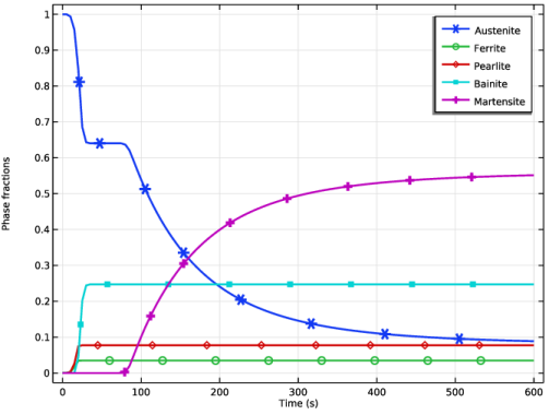
In the Settings window for 1D Plot Group, type Phase fractions at the billet center in the Label text field.
3
Click to expand the Title section. From the Title type list, choose None.
4
Locate the Plot Settings section.
5
Select the y-axis label checkbox. In the associated text field, type Phase fractions.
Point Graph 1
1
Right-click Phase fractions at the billet center and choose Point Graph.
2
3
In the Settings window for Point Graph, click Replace Expression in the upper-right corner of the y-Axis Data section. From the menu, choose Component 1 (comp1) > Austenite Decomposition > Austenite > audc.phase1.xiGp - Phase fraction - 1.
4
Click to expand the Coloring and Style section. From the Width list, choose 2.
5
Find the Line markers subsection. From the Marker list, choose Cycle.
6
From the Positioning list, choose Interpolated.
7
Click to expand the Legends section. Select the Show legends checkbox.
8
From the Legends list, choose Manual.
9
Point Graph 2
1
Right-click Point Graph 1 and choose Duplicate.
2
In the Settings window for Point Graph, locate the y-Axis Data section.
3
In the Expression text field, type audc.phase2.xiGp.
4
Locate the Legends section. In the table, enter the following settings:
Point Graph 3
1
In the Model Builder window, under Results > Phase fractions at the billet center right-click Point Graph 1 and choose Duplicate.
2
In the Settings window for Point Graph, locate the y-Axis Data section.
3
In the Expression text field, type audc.phase3.xiGp.
4
Locate the Legends section. In the table, enter the following settings:
Point Graph 4
1
Right-click Point Graph 1 and choose Duplicate.
2
In the Settings window for Point Graph, locate the y-Axis Data section.
3
In the Expression text field, type audc.phase4.xiGp.
4
Locate the Legends section. In the table, enter the following settings:
Point Graph 5
1
Right-click Point Graph 1 and choose Duplicate.
2
In the Settings window for Point Graph, locate the y-Axis Data section.
3
In the Expression text field, type audc.phase5.xiGp.
4
Locate the Legends section. In the table, enter the following settings:
Phase fractions at the billet surface
1
In the Model Builder window, right-click Phase fractions at the billet center and choose Duplicate.
2
In the Model Builder window, click Phase fractions at the billet center 1.
3
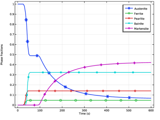
In the Settings window for 1D Plot Group, type Phase fractions at the billet surface in the Label text field.
Point Graph 1
1
In the Model Builder window, click Point Graph 1.
2
In the Settings window for Point Graph, locate the Selection section.
3
Click to select the  Activate Selection toggle button.
4
Point Graph 2
1
In the Model Builder window, click Point Graph 2.
2
In the Settings window for Point Graph, locate the Selection section.
3
Click to select the  Activate Selection toggle button.
4
Point Graph 3
1
In the Model Builder window, click Point Graph 3.
2
In the Settings window for Point Graph, locate the Selection section.
3
Click to select the  Activate Selection toggle button.
4
Point Graph 4
1
In the Model Builder window, click Point Graph 4.
2
In the Settings window for Point Graph, locate the Selection section.
3
Click to select the  Activate Selection toggle button.
4
Point Graph 5
1
In the Model Builder window, click Point Graph 5.
2
In the Settings window for Point Graph, locate the Selection section.
3
Click to select the  Activate Selection toggle button.
4
5
In the Phase fractions at the billet surface toolbar, click  Plot.
Axial stress profile
1
In the Results toolbar, click  1D Plot Group.
2
In the Settings window for 1D Plot Group, type Axial stress profile in the Label text field.
3
Locate the Data section. From the Time selection list, choose Last.
Line Graph 1
1
Right-click Axial stress profile and choose Line Graph.
2
3
In the Settings window for Line Graph, click Replace Expression in the upper-right corner of the y-Axis Data section. From the menu, choose Component 1 (comp1) > Solid Mechanics > Stress > Stress tensor (spatial frame) - N/m² > solid.sGpzz - Stress tensor, zz-component.
4
Locate the y-Axis Data section. From the Unit list, choose MPa.
5
Locate the x-Axis Data section. From the Parameter list, choose Expression.
6
In the Expression text field, type R.
7
Click to expand the Coloring and Style section. From the Width list, choose 2.
8
Click to expand the Quality section. In the Axial stress profile toolbar, click  Plot.
Mirror 3D 1
1
In the Results toolbar, click  More Datasets and choose Mirror 3D.
2
In the Settings window for Mirror 3D, locate the Plane Data section.
3
From the Plane list, choose XY-planes.
3D Plot Group 17
1
In the Results toolbar, click  3D Plot Group.
2
In the Settings window for 3D Plot Group, locate the Data section.
3
From the Dataset list, choose Mirror 3D 1.
4
Click to expand the Title section. From the Title type list, choose None.
5
Click to expand the Plot Array section. Select the Enable checkbox.
6
From the Array axis list, choose y.
7
From the Padding list, choose Absolute.
8
In the Padding length text field, type 0.05.
Axial stress
1
Right-click 3D Plot Group 17 and choose Surface.
2
In the Settings window for Surface, type Axial stress in the Label text field.
3
Click Replace Expression in the upper-right corner of the Expression section. From the menu, choose Component 1 (comp1) > Solid Mechanics > Stress > Stress tensor (spatial frame) - N/m² > solid.sGpzz - Stress tensor, zz-component.
4
Locate the Expression section. From the Unit list, choose MPa.
Equivalent plastic strain
1
Right-click Axial stress and choose Duplicate.
2
In the Settings window for Surface, type Equivalent plastic strain in the Label text field.
3
Click Replace Expression in the upper-right corner of the Expression section. From the menu, choose Component 1 (comp1) > Solid Mechanics > Strain > solid.epeGp - Equivalent plastic strain - 1.
4
Locate the Coloring and Style section. From the Color table list, choose Traffic.
Surface 1
1
In the Model Builder window, expand the Results > Martensite, 3D (audc) node.
2
Right-click Surface 1 and choose Copy.
Martensite phase fraction
1
In the Model Builder window, right-click 3D Plot Group 17 and choose Paste Surface.
2
In the Settings window for Surface, type Martensite phase fraction in the Label text field.