|
|
|
|
•
|
Phase transformation data is imported by selecting Import Phase Transformations in the physics interface context menu.
|
|
•
|
Phase material properties are imported by selecting Import Materials from the Materials context menu under Global Definitions or under Materials at the component level (not available in 0D).
|
|
1
|
|
2
|
|
3
|
Click Add.
|
|
4
|
Click
|
|
5
|
|
6
|
Click
|
|
1
|
|
2
|
|
3
|
Click
|
|
4
|
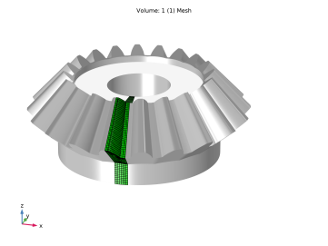
Browse to the model’s Application Libraries folder and double-click the file quenching_of_a_bevel_gear_mesh.mphbin.
|
|
5
|
Click
|
|
1
|
|
2
|
|
1
|
|
2
|
|
3
|
|
4
|
Click
|
|
5
|
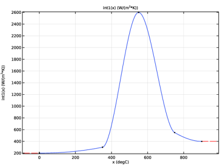
Browse to the model’s Application Libraries folder and double-click the file quenching_of_a_bevel_gear_htc.txt.
|
|
6
|
|
8
|
|
9
|
Locate the Interpolation and Extrapolation section. From the Interpolation list, choose Piecewise cubic.
|
|
10
|
Click
|
|
1
|
In the Model Builder window, expand the Heat Transfer in Solids (ht) node, then click Initial Values 1.
|
|
2
|
|
3
|
|
1
|
|
2
|
|
3
|
|
5
|
|
6
|
|
7
|
|
1
|
|
2
|
|
3
|
|
1
|
|
1
|
|
3
|
|
4
|
|
1
|
|
2
|
|
3
|
Browse to the model’s Application Libraries folder and double-click the file quenching_of_a_bevel_gear_JMatPro_general_steel.xml.
|
|
4
|
Click OK.
|
|
1
|
|
2
|
|
3
|
Click Create Compound Material in the upper-right corner of the section.
|
|
4
|
|
5
|
|
1
|
Right-click Component 1 (comp1) > Austenite Decomposition (audc) and choose Import Phase Transformations.
|
|
2
|
Browse to the model’s Application Libraries folder and double-click the file quenching_of_a_bevel_gear_JMatPro_general_steel.xml.
|
|
1
|
|
2
|
|
3
|
Locate the Mechanical Properties section. From the Isotropic hardening model list, choose Hardening function.
|
|
1
|
|
2
|
|
3
|
|
4
|
Locate the Mechanical Properties section. From the Isotropic hardening model list, choose Hardening function.
|
|
1
|
|
2
|
|
3
|
|
4
|
Locate the Mechanical Properties section. From the Isotropic hardening model list, choose Hardening function.
|
|
1
|
|
2
|
|
3
|
|
4
|
Locate the Mechanical Properties section. From the Isotropic hardening model list, choose Hardening function.
|
|
1
|
|
2
|
|
3
|
|
4
|
Locate the Mechanical Properties section. From the Isotropic hardening model list, choose Hardening function.
|
|
5
|
|
1
|
|
2
|
|
3
|
Find the Expression for remaining selection subsection. In the Volume reference temperature text field, type Tinit.
|
|
1
|
In the Model Builder window, under Component 1 (comp1) > Austenite Decomposition (audc) click General Steel, Austenite to Ferrite.
|
|
2
|
|
3
|
|
4
|
|
1
|
|
2
|
|
3
|
|
4
|
|
1
|
|
2
|
|
3
|
|
4
|
|
1
|
|
2
|
|
3
|
|
4
|
|
1
|
|
2
|
|
3
|
|
1
|
|
2
|
|
3
|
Click
|
|
4
|
|
5
|
Click OK.
|
|
6
|
|
8
|
Click
|
|
9
|
|
10
|
Click OK.
|
|
11
|