
|
|
|
|
1
|
|
2
|
In the Application Libraries window, select MEMS Module > Sensors > surface_micromachined_accelerometer_geom in the tree.
|
|
3
|
Click
|
|
1
|
|
2
|
|
1
|
|
2
|
Go to the Add Material window.
|
|
3
|
|
4
|
Right-click and choose Add to Component 1 (comp1).
|
|
5
|
|
1
|
|
2
|
|
1
|
|
2
|
|
3
|
|
1
|
|
2
|
|
3
|
|
4
|
|
5
|
Click OK.
|
|
6
|
|
7
|
|
8
|
|
9
|
Click OK.
|
|
1
|
In the Model Builder window, expand the Component 1 (comp1) > Moving Mesh node, then click Deforming Domain 1.
|
|
2
|
|
3
|
|
1
|
|
2
|
|
3
|
|
1
|
|
2
|
|
3
|
|
4
|
|
1
|
|
2
|
|
3
|
|
1
|
|
2
|
|
3
|
|
1
|
|
2
|
|
3
|
|
1
|
In the Model Builder window, expand the Component 1 (comp1) > Electrostatics (es) node, then click Charge Conservation in Solids 1.
|
|
2
|
|
3
|
|
1
|
|
1
|
|
2
|
|
3
|
|
4
|
|
5
|
|
1
|
|
2
|
|
3
|
|
4
|
|
5
|
|
1
|
|
2
|
|
3
|
|
1
|
|
2
|
|
3
|
|
4
|
|
5
|
|
1
|
|
2
|
|
3
|
|
4
|
|
5
|
|
1
|
|
2
|
|
3
|
|
4
|
Click
|
|
1
|
|
2
|
|
3
|
Click
|
|
5
|
|
6
|
Click
|
|
1
|
|
2
|
|
3
|
Click OK.
|
|
1
|
In the Model Builder window, expand the Study 1: Normal Operation node, then click Step 1: Stationary.
|
|
2
|
|
3
|
Select the Plot checkbox.
|
|
4
|
|
5
|
|
6
|
Click
|
|
7
|
Click
|
|
8
|
|
9
|
|
10
|
|
11
|
Click Add.
|
|
1
|
|
2
|
|
3
|
In the Model Builder window, expand the Study 1: Normal Operation > Solver Configurations > Solution 1 (sol1) > Dependent Variables 1 node, then click Spatial Mesh Displacement (comp1.spatial.disp).
|
|
4
|
|
5
|
|
6
|
In the Model Builder window, under Study 1: Normal Operation > Solver Configurations > Solution 1 (sol1) > Dependent Variables 1 click Displacement Field (comp1.u).
|
|
7
|
|
8
|
|
9
|
In the Model Builder window, under Study 1: Normal Operation > Solver Configurations > Solution 1 (sol1) > Dependent Variables 1 click Electric Potential (Material) (comp1.es.depV).
|
|
10
|
|
11
|
|
12
|
|
13
|
In the Model Builder window, under Study 1: Normal Operation > Solver Configurations > Solution 1 (sol1) > Dependent Variables 1 click Floating Potential (comp1.es.fp1.V0_ode).
|
|
14
|
|
15
|
|
16
|
|
17
|
In the Model Builder window, expand the Study 1: Normal Operation > Solver Configurations > Solution 1 (sol1) > Stationary Solver 1 > Segregated 1 node.
|
|
18
|
Right-click Study 1: Normal Operation > Solver Configurations > Solution 1 (sol1) > Stationary Solver 1 > Segregated 1 > Electric Potential and choose Move Down.
|
|
19
|
Right-click Study 1: Normal Operation > Solver Configurations > Solution 1 (sol1) > Stationary Solver 1 > Segregated 1 > Electric Potential and choose Move Down.
|
|
20
|
In the Model Builder window, under Study 1: Normal Operation > Solver Configurations > Solution 1 (sol1) > Stationary Solver 1 > Segregated 1 click Displacement Field.
|
|
21
|
|
22
|
|
23
|
In the Model Builder window, under Study 1: Normal Operation > Solver Configurations > Solution 1 (sol1) > Stationary Solver 1 > Segregated 1 click Spatial Mesh Displacement.
|
|
24
|
|
25
|
|
26
|
In the Model Builder window, under Study 1: Normal Operation > Solver Configurations > Solution 1 (sol1) > Stationary Solver 1 > Segregated 1 click Electric Potential.
|
|
27
|
|
28
|
|
29
|
|
1
|
|
2
|
|
3
|
|
4
|
|
1
|
|
2
|
|
3
|
|
4
|
Locate the Multiplane Data section. Find the x-planes subsection. From the Entry method list, choose Number of planes.
|
|
5
|
|
6
|
|
7
|
|
1
|
|
2
|
|
3
|
|
4
|
|
5
|
|
6
|
|
7
|
|
1
|
|
3
|
|
4
|
|
1
|
|
2
|
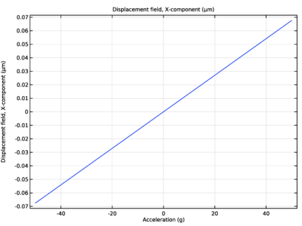
In the Settings window for 1D Plot Group, type Displacement vs. Acceleration in the Label text field.
|
|
3
|
Locate the Plot Settings section.
|
|
4
|
|
5
|
|
1
|
|
2
|
|
4
|
|
5
|
|
1
|
|
2
|
|
3
|
Click OK.
|
|
1
|
|
2
|
Go to the Add Study window.
|
|
3
|
|
4
|
Right-click and choose Add Study.
|
|
5
|
|
1
|
|
2
|
Select the Auxiliary sweep checkbox.
|
|
3
|
Click
|
|
5
|
Click
|
|
7
|
|
8
|
|
9
|
|
1
|
|
2
|
|
3
|
In the Model Builder window, expand the Study 2: Self Test > Solver Configurations > Solution 2 (sol2) > Dependent Variables 1 node, then click Spatial Mesh Displacement (comp1.spatial.disp).
|
|
4
|
|
5
|
|
6
|
In the Model Builder window, under Study 2: Self Test > Solver Configurations > Solution 2 (sol2) > Dependent Variables 1 click Displacement Field (comp1.u).
|
|
7
|
|
8
|
|
9
|
In the Model Builder window, under Study 2: Self Test > Solver Configurations > Solution 2 (sol2) > Dependent Variables 1 click Electric Potential (Material) (comp1.es.depV).
|
|
10
|
|
11
|
|
12
|
|
13
|
In the Model Builder window, under Study 2: Self Test > Solver Configurations > Solution 2 (sol2) > Dependent Variables 1 click Floating Potential (comp1.es.fp1.V0_ode).
|
|
14
|
|
15
|
|
16
|
|
17
|
In the Model Builder window, expand the Study 2: Self Test > Solver Configurations > Solution 2 (sol2) > Stationary Solver 1 > Segregated 1 node, then click Electric Potential.
|
|
18
|
|
19
|
|
20
|
In the Model Builder window, under Study 2: Self Test > Solver Configurations > Solution 2 (sol2) > Stationary Solver 1 > Segregated 1 click Displacement Field.
|
|
21
|
|
22
|
|
23
|
In the Model Builder window, under Study 2: Self Test > Solver Configurations > Solution 2 (sol2) > Stationary Solver 1 > Segregated 1 click Spatial Mesh Displacement.
|
|
24
|
|
25
|
|
26
|
|
1
|
|
2
|
|
3
|
|
4
|
|
5
|
|
1
|
|
2
|
|
3
|
|
4
|
|
5
|
|
6
|
|
1
|
|
2
|
|
3
|
|
4
|
|
5
|
|
6
|
|
7
|
|
1
|
|
2
|
|
3
|
|
1
|
|
3
|
|
4
|
|
5
|
|
6
|
|
7
|
|
1
|
|
2
|
|
3
|
Click OK.
|
|
1
|
|
2
|
In the Select Physics tree, select Structural Mechanics > Electromagnetics–Structure Interaction > Electromechanics > Electromechanics, Solid.
|
|
3
|
Click Add.
|
|
4
|
Click
|
|
5
|
|
6
|
Click
|
|
1
|
|
2
|
Browse to the model’s Application Libraries folder and double-click the file surface_micromachined_accelerometer_geom_subsequence.mph.
|
|
3
|
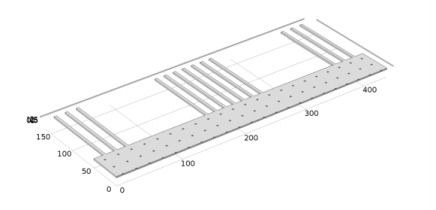
In the Load Part dialog, in the Select parts list, choose Proof mass with fingers, Spring and anchor, and Electrode array.
|
|
4
|
Click OK.
|
|
1
|
|
2
|
|
3
|
Click
|
|
4
|
Browse to the model’s Application Libraries folder and double-click the file surface_micromachined_accelerometer_parameters.txt.
|
|
1
|
|
2
|
|
3
|
Locate the Input Parameters section. In the table, enter the following settings:
|
|
4
|
Click
|
|
5
|
|
1
|
|
2
|
|
3
|
Locate the Input Parameters section. In the table, enter the following settings:
|
|
4
|
Click
|
|
1
|
|
2
|
|
3
|
Locate the Input Parameters section. In the table, enter the following settings:
|
|
4
|
Click
|
|
1
|
|
2
|
|
4
|
|
5
|
Click
|
|
6
|
|
1
|
|
2
|
In the Settings window for Part Instance, type Part Link: Sense Electrodes R in the Label text field.
|
|
3
|
Locate the Input Parameters section. In the table, enter the following settings:
|
|
4
|
Click
|
|
1
|
|
2
|
In the Settings window for Part Instance, type Part Link: Self Test Electrodes L 1 in the Label text field.
|
|
3
|
Locate the Input Parameters section. In the table, enter the following settings:
|
|
4
|
Click
|
|
6
|
Click
|
|
1
|
|
2
|
In the Settings window for Part Instance, type Part Link: Self Test Electrodes L 2 in the Label text field.
|
|
3
|
Locate the Input Parameters section. In the table, enter the following settings:
|
|
4
|
Click
|
|
1
|
|
2
|
In the Settings window for Part Instance, type Part Link: Self Test Electrodes R 1 in the Label text field.
|
|
3
|
Locate the Input Parameters section. In the table, enter the following settings:
|
|
4
|
Click
|
|
1
|
|
2
|
In the Settings window for Part Instance, type Part Link: Self Test Electrodes R 2 in the Label text field.
|
|
3
|
Locate the Input Parameters section. In the table, enter the following settings:
|
|
4
|
Click
|
|
5
|
|
1
|
|
2
|
|
3
|
|
4
|
|
5
|
|
6
|
|
7
|
|
8
|
Click to expand the Layers section. In the table, enter the following settings:
|
|
9
|
Click
|
|
10
|
|
11
|
|
12
|
|
13
|
|
14
|
|
15
|
|
1
|
|
2
|
|
3
|
|
1
|
|
2
|
|
1
|
|
2
|
|
3
|
|
4
|
|
5
|
Click
|
|
1
|
|
2
|
|
4
|
Click
|
|
1
|
|
2
|
|
4
|
Click New Cumulative Selection.
|
|
5
|
|
6
|
Click OK.
|
|
7
|
|
8
|
Click New Cumulative Selection.
|
|
9
|
|
10
|
Click OK.
|
|
11
|
|
1
|
|
2
|
|
4
|
Locate the Boundary Selections section. In the table, enter the following settings:
|
|
1
|
|
2
|
|
4
|
Locate the Boundary Selections section. In the table, enter the following settings:
|
|
1
|
|
2
|
|
4
|
Locate the Boundary Selections section. Click to select the first row in the table.
|
|
5
|
Click New Cumulative Selection.
|
|
6
|
|
7
|
Click OK.
|
|
1
|
|
2
|
|
4
|
Locate the Boundary Selections section. Click to select the first row in the table.
|
|
5
|
Click New Cumulative Selection.
|
|
6
|
|
7
|
Click OK.
|
|
1
|
|
2
|
|
4
|
|
5
|
|
6
|
Click OK.
|
|
7
|
|
1
|
In the Model Builder window, expand the Component 1 (comp1) > Geometry 1 > Cumulative Selections node, then click Component 1 (comp1) > Geometry 1 > Part Link: Self Test Electrodes L 2 (pi7).
|
|
2
|
|
4
|
Locate the Boundary Selections section. In the table, enter the following settings:
|
|
1
|
|
2
|
|
5
|
|
6
|
|
7
|
Click OK.
|
|
8
|
|
1
|
|
2
|
|
4
|
Locate the Boundary Selections section. In the table, enter the following settings:
|
|
1
|
In the Model Builder window, collapse the Component 1 (comp1) > Geometry 1 > Cumulative Selections node.
|
|
2
|
|
1
|
|
2
|
|
3
|
|
4
|
|
5
|
|
6
|
|
7
|
|
1
|
|
2
|
|
3
|
|
4
|
|
5
|
|
6
|
|
1
|
|
2
|
|
3
|
|
4
|
|
5
|
|
6
|