|
|
|

|
520 μm
|
1780 μm
|
1780 μm
|
|
|
40 μm
|
400 μm
|
3.95 μm
|
|
|
100 μm
|
2960 μm
|
2960 μm
|
|
1
|
|
2
|
In the Select Physics tree, select Structural Mechanics > Fluid–Structure Interaction > Thin-Film Damping > Solid–Thin-Film Damping.
|
|
3
|
Click Add.
|
|
4
|
Click
|
|
5
|
|
6
|
Click
|
|
1
|
|
2
|
|
3
|
Locate the Parameters section. In the table, enter the following settings:
|
|
1
|
|
2
|
|
3
|
Locate the Parameters section. In the table, enter the following settings:
|
|
1
|
|
2
|
|
3
|
|
1
|
|
2
|
|
3
|
|
4
|
|
5
|
|
1
|
|
2
|
|
3
|
|
4
|
|
5
|
|
6
|
|
7
|
|
8
|
|
1
|
|
2
|
|
3
|
|
4
|
|
5
|
|
6
|
|
7
|
|
8
|
|
9
|
Click
|
|
10
|
|
1
|
|
2
|
Go to the Add Material window.
|
|
3
|
|
4
|
Click the Add to Component button in the window toolbar.
|
|
5
|
|
1
|
|
2
|
Click in the Graphics window and then press Ctrl+A to select all domains.
|
|
3
|
|
4
|
|
1
|
|
1
|
|
3
|
|
4
|
|
1
|
In the Model Builder window, under Component 1 (comp1) > Thin-Film Flow (tff) click Fluid-Film Properties 1.
|
|
2
|
|
3
|
Click Make All Model Inputs Editable in the upper-right corner of the section.
|
|
4
|
|
5
|
|
6
|
Locate the Fluid Properties section. From the μ list, choose User defined. In the associated text field, type mu.
|
|
7
|
Locate the Film Flow Model section. From the Film flow model list, choose Rarefied-total accommodation.
|
|
8
|
|
9
|
|
1
|
|
2
|
In the Settings window for Integration, type Bottom Surface Integration Operator in the Label text field.
|
|
3
|
|
4
|
|
1
|
|
2
|
In the Settings window for Integration, type Top Surface Integration Operator in the Label text field.
|
|
3
|
|
4
|
|
1
|
|
2
|
|
3
|
Locate the Variables section. In the table, enter the following settings:
|
|
1
|
|
2
|
|
1
|
|
2
|
Go to the Add Physics window.
|
|
3
|
In the tree, select Structural Mechanics > Fluid–Structure Interaction > Thin-Film Damping > Solid–Thin-Film Damping.
|
|
4
|
Click the Add to Component 2 button in the window toolbar.
|
|
5
|
|
1
|
|
2
|
|
1
|
|
2
|
|
3
|
|
4
|
|
1
|
|
2
|
|
3
|
|
4
|
|
5
|
|
6
|
|
7
|
Click
|
|
8
|
|
1
|
|
2
|
Go to the Add Material window.
|
|
3
|
|
4
|
Click the Add to Component button in the window toolbar.
|
|
5
|
|
1
|
|
2
|
|
4
|
|
1
|
|
2
|
|
4
|
|
1
|
|
2
|
Click in the Graphics window and then press Ctrl+A to select both domains.
|
|
3
|
|
4
|
|
1
|
|
1
|
|
3
|
|
4
|
|
1
|
In the Model Builder window, under Component 2 (comp2) > Thin-Film Flow 2 (tff2) click Fluid-Film Properties 1.
|
|
2
|
|
3
|
Click Make All Model Inputs Editable in the upper-right corner of the section.
|
|
4
|
|
5
|
|
6
|
Locate the Fluid Properties section. From the μ list, choose User defined. In the associated text field, type mu.
|
|
7
|
Locate the Film Flow Model section. From the Film flow model list, choose Rarefied-total accommodation.
|
|
8
|
|
9
|
|
1
|
|
2
|
In the Settings window for Integration, type Bottom Surface Integration Operator in the Label text field.
|
|
3
|
|
4
|
|
1
|
|
2
|
In the Settings window for Integration, type Top Surface Integration Operator in the Label text field.
|
|
3
|
|
4
|
|
1
|
|
2
|
|
3
|
Locate the Variables section. In the table, enter the following settings:
|
|
1
|
In the Model Builder window, under Component 2 (comp2) > Multiphysics click Structure–Thin-Film Flow Interaction 2 (stfi2).
|
|
1
|
|
2
|
|
3
|
Click the Custom button.
|
|
4
|
|
5
|
|
6
|
|
7
|
|
8
|
|
1
|
|
2
|
|
3
|
Click
|
|
1
|
|
2
|
|
3
|
|
4
|
|
1
|
|
2
|
|
3
|
In the Model Builder window, expand the Study 1 > Solver Configurations > Solution 1 (sol1) > Time-Dependent Solver 1 node.
|
|
4
|
|
1
|
|
1
|
|
2
|
|
3
|
|
1
|
|
2
|
Go to the Result Templates window.
|
|
3
|
In the tree, select Study 1/Parametric Solutions 1 (4) (sol2) > Solid Mechanics 2 > Displacement (solid2).
|
|
4
|
Click the Add Result Template button in the window toolbar.
|
|
5
|
|
1
|
|
2
|
|
3
|
|
4
|
|
5
|
|
1
|
|
2
|
|
1
|
|
2
|
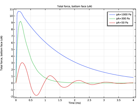
In the Settings window for 1D Plot Group, type Total Force on Bottom Surface (3D) in the Label text field.
|
|
3
|
|
4
|
Locate the Plot Settings section.
|
|
5
|
|
1
|
|
2
|
|
4
|
Click to expand the Coloring and Style section. Click to expand the Legends section. Find the Include subsection. Clear the Description checkbox.
|
|
5
|
|
1
|
|
2
|
|
3
|
|
4
|
Locate the Plot Settings section.
|
|
5
|
|
6
|
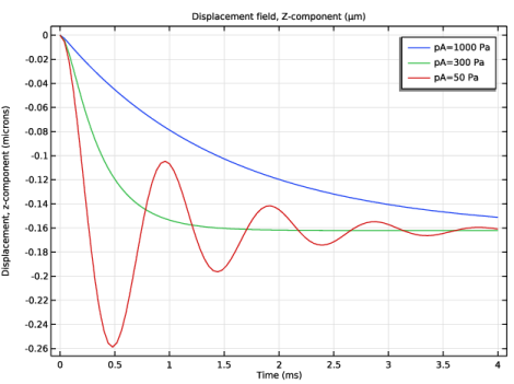
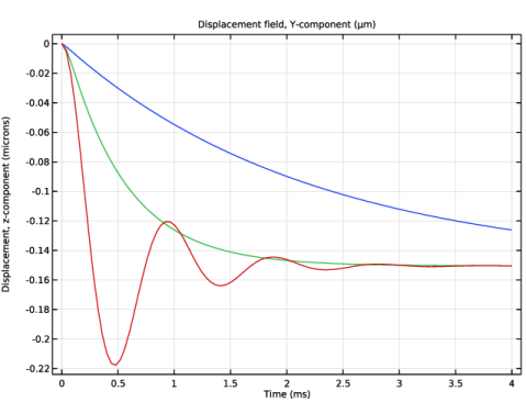
Select the y-axis label checkbox. In the associated text field, type Displacement, z-component (microns).
|
|
1
|
|
3
|
In the Settings window for Point Graph, click Replace Expression in the upper-right corner of the y-Axis Data section. From the menu, choose Component 1 (comp1) > Solid Mechanics > Displacement > Displacement field - m > w - Displacement field, Z-component.
|
|
4
|
|
5
|
Select the Show legends checkbox.
|
|
6
|
|
1
|
|
2
|
|
1
|
|
2
|
In the Settings window for 1D Plot Group, type Total Force on Bottom Surface (2D) in the Label text field.
|
|
3
|
|
4
|
Locate the Plot Settings section.
|
|
5
|
|
6
|
|
1
|
|
2
|
|
4
|
|
5
|
|
1
|
|
2
|
|
3
|
|
4
|
Locate the Plot Settings section.
|
|
5
|
|
6
|
Select the y-axis label checkbox. In the associated text field, type Displacement, z-component (microns).
|
|
1
|
|
3
|
In the Settings window for Point Graph, click Replace Expression in the upper-right corner of the y-Axis Data section. From the menu, choose Component 2 (comp2) > Solid Mechanics 2 > Displacement > Displacement field - m > v2 - Displacement field, Y-component.
|
|
4
|
|
5
|
|
6
|
Select the Show legends checkbox.
|