PDF

Surface Acoustic Wave Velocity Calculations from a Unit Cell
Introduction
FEM simulations can be used to obtain the surface acoustic wave (SAW) velocity and related parameters, such as the squared electromechanical coupling coefficient, or k2, and reflectivity, or kp, for different configurations. Such parameters are used as input for various analytical and semi-analytical methods of SAW device design, for example, the Delta-Function model and the COM method. The typical setup for FEM simulations is a unit-cell model encompassing one wavelength with periodic boundary conditions and an Eigenfrequency study. This tutorial investigates unit cells of 128 YX-cut LiNbO3 crystal with the size chosen for a center frequency of about 433 MHz. The first unit cell studied has a free surface, that is, a surface without IDT or electric terminals. The second unit cell has IDT, that is, two grounded aluminum electrodes. The third unit cell studied has a fully grounded top surface.
Model Definition
To model the unit cell, a Piezoelectricity interface with a Periodic Condition feature are used. To define the crystal cut, a Rotated System feature is used. In addition, a Perfectly Matched Layer is used to efficiently model SAWs propagating in thick substrates. To simulate the SAW phenomenon, the Eigenfrequency study is performed to solve for two eigenfrequencies around 433 MHz.
The geometric parameters are summarized in the first table in the Modeling Instructions section. The parameterized geometry facilitates design optimization. The model geometry includes three unit cells with free surface, IDT, and a grounded bottom surface, as shown in Figure 1.
Figure 1: The model geometry includes three unit cells with free surface (left), IDT (center), and a grounded bottom surface (right).
Note that it is necessary to enable the Out-of-plane mode extension (time-harmonic) in the Solid Mechanics interface for the 2D component to obtain results for all three displacement components. Otherwise, one displacement component and its derivatives would be zero.
From an Eigenfrequency study, f1 (resonance) and f2 (anti-resonance) are obtained. In the case of free surface or grounded, f1 and f2 should be equal. The related parameters cfree, cIDT, cgrounded, k2, and kp can be calculated in results processing using a Global Evaluation feature. Simply define the parameter and the expressions to be evaluated. The SAW velocity for the free surface is defined as
with f1,free and f2,free denoting the resonance and anti-resonance frequencies, respectively.
Similarly, in the case with IDT, the velocity is defined as
with f1,IDT and f2,IDT denoting the resonance and anti-resonance frequencies, respectively. Lastly, in the grounded case, the velocity is defined as
with f1,IDT and f2,IDT denoting the resonance and anti-resonance frequencies, respectively. The squared electromechanical coupling coefficient, k2, is defined by
and the reflectivity, kp, is defined by
Results and Discussion
Based on the results of the Eigenfrequency studies for each case, the parameters of interest are calculated using a Global Evaluation feature. They are summarized in Table 1.
Unit-cell modeling shown in this tutorial can be performed as verification before moving forward for more complex, full device configurations. This approach can give accurate results for different configurations, including double-electrode designs, SPUDT (unidirectional IDTs), trapezoid-shaped electrodes, multilayered structures, and so on. This approach is also valid for structures other than IDTs: all kinds of reflectors, different projections, grooves, and so on. The FEM formulation solves for the SAW velocity regardless of the IDT size and grating pattern, and automatically includes parameters such as electrode mass loading, internal reflections, scattering, and BAW radiation.
Provided that the model setup is correct, all the obtained parameters are thoroughly dependent on the material data used. That said, one has to be very careful with the material properties of a piezoelectric crystal and IDT, and has to ensure they are consistent with the experimental setup. Any notable discrepancies may end up in a different phase velocity and thus a different resonance frequency. The latter may significantly affect any frequency response of a complex SAW device. This is another reason to run a unit-cell model for verification, especially when new untested set of constants are involved.
Every Eigenfrequency study here is designed to return two SAW modes. This is achieved via a good initial guess specified in the Search for eigenfrequencies around shift text field. When performing your own simulation, you might need to adjust this initial guess. It might be a good idea to manually investigate all the obtained modes to ensure that they are of the SAW class.
To evaluate the aforementioned parameters in the most automated way, one needs to reach every solution and every mode within that solution independent of the dataset used. This can be implemented via a special withsol operator with an additional setind-argument. For example, calling withsol('sol3',real(freq),setind(lambda,2)) will return the real part of the second eigenfrequency obtained in the third study. More information can be found in the COMSOL Multiphysics Reference Manual; search for “Built-In Operators.”
Reference
1. K. Hashimoto, Surface Acoustic Wave Devices in Telecommunications: Modelling and Simulation, Springer-Verlag Berlin, Heidelberg, 2000; DOI: doi.org/10.1007/978-3-662-04223-6.
Application Library path: MEMS_Module/Piezoelectric_Devices/saw_velocity_calculation
Modeling Instructions
From the File menu, choose New.
New
In the New window, click  Model Wizard.
Start by creating a new 2D model with three Piezoelectricity multiphysics interfaces for modeling free, IDT and grounded unit cells. Also select Eigenfrequency for the first study.
Model Wizard
1
In the Model Wizard window, click  2D.
2
In the Select Physics tree, select AC/DC > Electromagnetics and Mechanics > Piezoelectricity > Piezoelectricity, Solid.
3
Click Add.
4
Click Add.
5
Click Add.
6
Click  Study.
7
In the Select Study tree, select Preset Studies for Selected Multiphysics > Eigenfrequency.
8
Define and specify the parameters of the model.
Global Definitions
Parameters 1
1
In the Model Builder window, under Global Definitions click Parameters 1.
2
In the Settings window for Parameters, locate the Parameters section.
3
Create the geometry for the free unit cell. Use microns as the geometry unit.
Geometry 1
1
In the Model Builder window, under Component 1 (comp1) click Geometry 1.
2
In the Settings window for Geometry, locate the Units section.
3
From the Length unit list, choose µm.
Rectangle 1 (r1)
1
In the Geometry toolbar, click  Rectangle.
2
In the Settings window for Rectangle, locate the Size and Shape section.
3
In the Width text field, type lambdaD.
4
In the Height text field, type h_sub.
5
Click to expand the Layers section. In the table, enter the following settings:
6
Click  Build Selected.
Create the geometry for the unit cell with IDT.
Copy 1 (copy1)
1
In the Geometry toolbar, click  Transforms and choose Copy.
2
3
In the Settings window for Copy, locate the Displacement section.
4
In the x text field, type lambdaD*2.
5
Click  Build Selected.
Rectangle 2 (r2)
1
In the Geometry toolbar, click  Rectangle.
2
In the Settings window for Rectangle, locate the Size and Shape section.
3
In the Width text field, type l_el.
4
In the Height text field, type h_el.
5
Locate the Position section. In the x text field, type lambdaD*2+lambdaD/8.
6
In the y text field, type h_sub.
7
Click  Build Selected.
Array 1 (arr1)
1
In the Geometry toolbar, click  Transforms and choose Array.
2
3
In the Settings window for Array, locate the Size section.
4
From the Array type list, choose Linear.
5
In the Size text field, type 2.
6
Locate the Displacement section. In the x text field, type lambdaD/2.
7
Click  Build Selected.
Create the geometry for the grounded unit cell.
Copy 2 (copy2)
1
In the Geometry toolbar, click  Transforms and choose Copy.
2
Click the  Select Box button in the Graphics toolbar.
3
4
In the Settings window for Copy, locate the Displacement section.
5
In the x text field, type lambdaD*4.
6
Click  Build Selected.
Define selections for the various domains and boundaries.
Definitions
Substrate
1
In the Definitions toolbar, click  Explicit.
2
In the Settings window for Explicit, type Substrate in the Label text field.
3
PML
1
In the Definitions toolbar, click  Explicit.
2
In the Settings window for Explicit, type PML in the Label text field.
3
IDT
1
In the Definitions toolbar, click  Explicit.
2
In the Settings window for Explicit, type IDT in the Label text field.
3
Free Unit Cell
1
In the Definitions toolbar, click  Explicit.
2
In the Settings window for Explicit, type Free Unit Cell in the Label text field.
3
Click the  Select Box button in the Graphics toolbar.
4
IDT Unit Cell
1
In the Definitions toolbar, click  Explicit.
2
In the Settings window for Explicit, type IDT Unit Cell in the Label text field.
3
Click the  Select Box button in the Graphics toolbar.
4
Grounded Unit Cell
1
In the Definitions toolbar, click  Explicit.
2
In the Settings window for Explicit, type Grounded Unit Cell in the Label text field.
3
Click the  Select Box button in the Graphics toolbar.
4
Periodic
1
In the Definitions toolbar, click  Explicit.
2
In the Settings window for Explicit, locate the Input Entities section.
3
From the Geometric entity level list, choose Boundary.
4
In the Label text field, type Periodic.
5
Fixed
1
In the Definitions toolbar, click  Explicit.
2
In the Settings window for Explicit, type Fixed in the Label text field.
3
Locate the Input Entities section. From the Geometric entity level list, choose Boundary.
4
Define operators that could be useful in results processing.
Maximum 1 (maxop1)
1
In the Definitions toolbar, click  Nonlocal Couplings and choose Maximum.
2
In the Settings window for Maximum, locate the Source Selection section.
3
From the Selection list, choose Free Unit Cell.
Maximum 2 (maxop2)
1
In the Definitions toolbar, click  Nonlocal Couplings and choose Maximum.
2
In the Settings window for Maximum, locate the Source Selection section.
3
From the Selection list, choose IDT Unit Cell.
Maximum 3 (maxop3)
1
In the Definitions toolbar, click  Nonlocal Couplings and choose Maximum.
2
In the Settings window for Maximum, locate the Source Selection section.
3
From the Selection list, choose Grounded Unit Cell.
Define a rotated system for the 128 YX-cut lithium niobate.
Rotated System 2 (sys2)
1
In the Definitions toolbar, click  Coordinate Systems and choose Rotated System.
2
In the Settings window for Rotated System, locate the Rotation section.
3
From the Input method list, choose General rotation.
4
Find the Euler angles subsection. In the β text field, type -38[deg]-90[deg].
Define a perfectly matched layer.
Perfectly Matched Layer 1 (pml1)
1
In the Definitions toolbar, click  Perfectly Matched Layer.
2
In the Settings window for Perfectly Matched Layer, locate the Domain Selection section.
3
From the Selection list, choose PML.
Add materials and assign the domains they belong to.
Add Material
1
In the Materials toolbar, click  Add Material to open the Add Material window.
2
Go to the Add Material window.
3
In the tree, select MEMS > Metals > Al - Aluminum.
4
Click the Add to Component button in the window toolbar.
Materials
Al - Aluminum (mat1)
1
In the Settings window for Material, locate the Geometric Entity Selection section.
2
From the Selection list, choose IDT.
Add Material
1
Go to the Add Material window.
2
In the tree, select Piezoelectric > Lithium Niobate.
3
Click the Add to Component button in the window toolbar.
4
In the Materials toolbar, click  Add Material to close the Add Material window.
Materials
Lithium Niobate (mat2)
1
In the Settings window for Material, locate the Geometric Entity Selection section.
2
From the Selection list, choose Substrate.
Specify the settings for the Electrostatics and Solid Mechanics interfaces in the free unit cell.
Electrostatics (es)
1
In the Model Builder window, under Component 1 (comp1) click Electrostatics (es).
2
In the Settings window for Electrostatics, locate the Domain Selection section.
3
From the Selection list, choose Free Unit Cell.
4
Locate the Thickness section. In the d text field, type W.
Periodic Condition 1
1
In the Physics toolbar, click  Boundaries and choose Periodic Condition.
2
In the Settings window for Periodic Condition, locate the Boundary Selection section.
3
From the Selection list, choose Periodic.
Solid Mechanics (solid)
1
In the Model Builder window, under Component 1 (comp1) click Solid Mechanics (solid).
2
In the Settings window for Solid Mechanics, locate the Domain Selection section.
3
From the Selection list, choose Free Unit Cell.
4
Locate the 2D Approximation section. Select the Out-of-plane mode extension (time-harmonic) checkbox.
5
Locate the Thickness section. In the d text field, type W.
Piezoelectric Material 1
1
In the Model Builder window, under Component 1 (comp1) > Solid Mechanics (solid) click Piezoelectric Material 1.
2
In the Settings window for Piezoelectric Material, locate the Coordinate System Selection section.
3
From the Coordinate system list, choose Rotated System 2 (sys2).
Periodic Condition 1
1
In the Physics toolbar, click  Boundaries and choose Periodic Condition.
2
In the Settings window for Periodic Condition, locate the Boundary Selection section.
3
From the Selection list, choose Periodic.
Fixed Constraint 1
1
In the Physics toolbar, click  Boundaries and choose Fixed Constraint.
2
In the Settings window for Fixed Constraint, locate the Boundary Selection section.
3
From the Selection list, choose Fixed.
Specify the settings for the Electrostatics and Solid Mechanics interfaces in the IDT unit cell.
Electrostatics 2 (es2)
1
In the Model Builder window, under Component 1 (comp1) click Electrostatics 2 (es2).
2
In the Settings window for Electrostatics, locate the Domain Selection section.
3
From the Selection list, choose IDT Unit Cell.
4
Locate the Thickness section. In the d text field, type W.
Boundary Terminal 1
In the Physics toolbar, click  Boundaries and choose Boundary Terminal.
Periodic Condition 1
1
In the Physics toolbar, click  Boundaries and choose Periodic Condition.
2
In the Settings window for Periodic Condition, locate the Boundary Selection section.
3
From the Selection list, choose Periodic.
Charge Conservation, Piezoelectric 1
1
In the Model Builder window, click Charge Conservation, Piezoelectric 1.
2
In the Settings window for Charge Conservation, Piezoelectric, locate the Domain Selection section.
3
From the Selection list, choose Substrate.
Boundary Terminal 1
1
In the Model Builder window, click Boundary Terminal 1.
2
In the Settings window for Boundary Terminal, locate the Boundary Selection section.
3
Click  Paste Selection.
4
In the Paste Selection dialog, type 19 in the Selection text field.
5
6
In the Settings window for Boundary Terminal, locate the Terminal section.
7
From the Terminal type list, choose Voltage.
Ground 1
1
In the Physics toolbar, click  Boundaries and choose Ground.
2
In the Settings window for Ground, locate the Boundary Selection section.
3
Click  Paste Selection.
4
In the Paste Selection dialog, type 14 in the Selection text field.
5
Solid Mechanics 2 (solid2)
1
In the Model Builder window, under Component 1 (comp1) click Solid Mechanics 2 (solid2).
2
In the Settings window for Solid Mechanics, locate the Domain Selection section.
3
From the Selection list, choose IDT Unit Cell.
4
Locate the 2D Approximation section. Select the Out-of-plane mode extension (time-harmonic) checkbox.
5
Locate the Thickness section. In the d text field, type W.
Piezoelectric Material 1
1
In the Model Builder window, under Component 1 (comp1) > Solid Mechanics 2 (solid2) click Piezoelectric Material 1.
2
In the Settings window for Piezoelectric Material, locate the Domain Selection section.
3
From the Selection list, choose Substrate.
4
Locate the Coordinate System Selection section. From the Coordinate system list, choose Rotated System 2 (sys2).
Periodic Condition 1
1
In the Physics toolbar, click  Boundaries and choose Periodic Condition.
2
In the Settings window for Periodic Condition, locate the Boundary Selection section.
3
From the Selection list, choose Periodic.
Fixed Constraint 1
1
In the Physics toolbar, click  Boundaries and choose Fixed Constraint.
2
In the Settings window for Fixed Constraint, locate the Boundary Selection section.
3
From the Selection list, choose Fixed.
Specify the settings for the Electrostatics and Solid Mechanics interfaces in the grounded unit cell.
Electrostatics 3 (es3)
1
In the Model Builder window, under Component 1 (comp1) click Electrostatics 3 (es3).
2
In the Settings window for Electrostatics, locate the Domain Selection section.
3
From the Selection list, choose Grounded Unit Cell.
4
Locate the Thickness section. In the d text field, type W.
Periodic Condition 1
1
In the Physics toolbar, click  Boundaries and choose Periodic Condition.
2
In the Settings window for Periodic Condition, locate the Boundary Selection section.
3
From the Selection list, choose Periodic.
Ground 1
1
In the Physics toolbar, click  Boundaries and choose Ground.
2
Solid Mechanics 3 (solid3)
1
In the Model Builder window, under Component 1 (comp1) click Solid Mechanics 3 (solid3).
2
In the Settings window for Solid Mechanics, locate the Domain Selection section.
3
From the Selection list, choose Grounded Unit Cell.
4
Locate the 2D Approximation section. Select the Out-of-plane mode extension (time-harmonic) checkbox.
5
Locate the Thickness section. In the d text field, type W.
Piezoelectric Material 1
1
In the Model Builder window, under Component 1 (comp1) > Solid Mechanics 3 (solid3) click Piezoelectric Material 1.
2
In the Settings window for Piezoelectric Material, locate the Coordinate System Selection section.
3
From the Coordinate system list, choose Rotated System 2 (sys2).
Periodic Condition 1
1
In the Physics toolbar, click  Boundaries and choose Periodic Condition.
2
In the Settings window for Periodic Condition, locate the Boundary Selection section.
3
From the Selection list, choose Periodic.
Fixed Constraint 1
1
In the Physics toolbar, click  Boundaries and choose Fixed Constraint.
2
In the Settings window for Fixed Constraint, locate the Boundary Selection section.
3
From the Selection list, choose Fixed.
Create the mesh for the free, IDT and grounded unit cells.
Mesh Free
1
In the Model Builder window, under Component 1 (comp1) click Mesh 1.
2
In the Settings window for Mesh, type Mesh Free in the Label text field.
3
Locate the Sequence Type section. From the list, choose User-controlled mesh.
Distribution 1, Free Triangular 1, Identical Mesh 1, Identical Mesh 2, Identical Mesh 3, Mapped 1
1
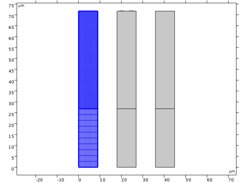
In the Model Builder window, under Component 1 (comp1) > Mesh Free, Ctrl-click to select Identical Mesh 1, Identical Mesh 2, Identical Mesh 3, Distribution 1, Free Triangular 1, and Mapped 1.
2
Size
1
In the Settings window for Size, locate the Element Size section.
2
Click the Custom button.
3
Locate the Element Size Parameters section. In the Maximum element size text field, type lambdaD/20.
4
In the Minimum element size text field, type lambdaD/20.
Edge 1
1
In the Mesh toolbar, click  More Generators and choose Edge.
2
Distribution 1
1
Right-click Edge 1 and choose Distribution.
2
3
In the Settings window for Distribution, locate the Distribution section.
4
In the Number of elements text field, type 10.
Mapped 1
1
In the Mesh toolbar, click  Mapped.
2
In the Settings window for Mapped, locate the Domain Selection section.
3
From the Geometric entity level list, choose Domain.
4
5
Click  Build All.
Mesh IDT
1
In the Mesh toolbar, click Add Mesh and choose Add Mesh.
2
In the Settings window for Mesh, type Mesh IDT in the Label text field.
3
Locate the Sequence Type section. From the list, choose User-controlled mesh.
Distribution 1, Free Triangular 1, Identical Mesh 1, Identical Mesh 2, Identical Mesh 3, Mapped 1
1
In the Model Builder window, under Component 1 (comp1) > Meshes > Mesh IDT, Ctrl-click to select Identical Mesh 1, Identical Mesh 2, Identical Mesh 3, Distribution 1, Free Triangular 1, and Mapped 1.
2
Size
1
In the Settings window for Size, locate the Element Size section.
2
Click the Custom button.
3
Locate the Element Size Parameters section. In the Maximum element size text field, type lambdaD/20.
4
In the Minimum element size text field, type lambdaD/20.
Edge 1
1
In the Mesh toolbar, click  More Generators and choose Edge.
2
Distribution 1
1
Right-click Edge 1 and choose Distribution.
2
3
In the Settings window for Distribution, locate the Distribution section.
4
In the Number of elements text field, type 10.
Mapped 1
1
In the Mesh toolbar, click  Mapped.
2
In the Settings window for Mapped, locate the Domain Selection section.
3
From the Geometric entity level list, choose Domain.
4
Click  Paste Selection.
5
In the Paste Selection dialog, type 5 6 in the Selection text field.
6
Distribution 1
1
Right-click Mapped 1 and choose Distribution.
2
In the Settings window for Distribution, locate the Boundary Selection section.
3
Click  Paste Selection.
4
In the Paste Selection dialog, type 16 21 in the Selection text field.
5
6
In the Settings window for Distribution, locate the Distribution section.
7
In the Number of elements text field, type 2.
8
Click  Build Selected.
Edge 2
1
In the Mesh toolbar, click  More Generators and choose Edge.
2
In the Settings window for Edge, locate the Boundary Selection section.
3
Click  Paste Selection.
4
In the Paste Selection dialog, type 12 17 22 in the Selection text field.
5
6
In the Settings window for Edge, click  Build Selected.
Copy Edge 1
1
In the Model Builder window, right-click Mesh IDT and choose Copying Operations > Copy Edge.
2
In the Settings window for Copy Edge, locate the Source Boundaries section.
3
Click  Paste Selection.
4
In the Paste Selection dialog, type 12 14 17 19 22 in the Selection text field.
5
6
In the Settings window for Copy Edge, locate the Destination Boundaries section.
7
Click to select the  Activate Selection toggle button.
8
Click  Paste Selection.
9
In the Paste Selection dialog, type 9 11 in the Selection text field.
10
11
In the Settings window for Copy Edge, click  Build Selected.
Mapped 2
1
In the Mesh toolbar, click  Mapped.
2
In the Settings window for Mapped, locate the Domain Selection section.
3
From the Geometric entity level list, choose Domain.
4
Click  Paste Selection.
5
In the Paste Selection dialog, type 3 4 in the Selection text field.
6
Distribution 1
1
Right-click Mapped 2 and choose Distribution.
2
In the Settings window for Distribution, locate the Boundary Selection section.
3
Click  Paste Selection.
4
In the Paste Selection dialog, type 8 in the Selection text field.
5
6
In the Settings window for Distribution, locate the Distribution section.
7
In the Number of elements text field, type 10.
Mapped 2
In the Model Builder window, right-click Mapped 2 and choose Build All.
Mesh Free
In the Model Builder window, under Component 1 (comp1) > Meshes right-click Mesh Free and choose Duplicate.
Mesh Grounded
In the Settings window for Mesh, type Mesh Grounded in the Label text field.
Edge 1
1
In the Model Builder window, expand the Mesh Grounded node, then click Edge 1.
2
In the Settings window for Edge, locate the Boundary Selection section.
3
Click  Clear Selection.
4
Distribution 1
1
In the Model Builder window, expand the Edge 1 node, then click Distribution 1.
2
In the Settings window for Distribution, locate the Boundary Selection section.
3
Click  Clear Selection.
4
Mapped 1
1
In the Model Builder window, under Component 1 (comp1) > Meshes > Mesh Grounded click Mapped 1.
2
In the Settings window for Mapped, locate the Domain Selection section.
3
Click  Clear Selection.
4
5
Click  Build All.
Free
1
In the Model Builder window, click Study 1.
2
In the Settings window for Study, type Free in the Label text field.
Set up Eigenfrequency study to search around f_0 MHz.
Step 1: Eigenfrequency
1
In the Model Builder window, under Free click Step 1: Eigenfrequency.
2
In the Settings window for Eigenfrequency, locate the Study Settings section.
3
Select the Desired number of eigenfrequencies checkbox. In the associated text field, type 2.
4
From the Unit list, choose MHz.
5
In the Search for eigenfrequencies around shift text field, type f_0.
6
Locate the Physics and Variables Selection section. In the Solve for column of the table, under Component 1 (comp1), clear the checkboxes for Electrostatics 2 (es2), Solid Mechanics 2 (solid2), Electrostatics 3 (es3), and Solid Mechanics 3 (solid3).
7
In the Solve for column of the table, under Component 1 (comp1) > Multiphysics, clear the checkboxes for Piezoelectricity 2 (pze2) and Piezoelectricity 3 (pze3).
Instead of using all geometric entities, select only Free Unit Cell.
Solution 1 (sol1)
1
In the Study toolbar, click  Show Default Solver.
2
In the Model Builder window, expand the Solution 1 (sol1) node, then click Compile Equations: Eigenfrequency.
3
In the Settings window for Compile Equations, locate the Geometric Entity Selection section.
4
From the Use entities list, choose Selected.
5
Under Selections, click  Add.
6
In the Add dialog, select Free Unit Cell in the Selections list.
7
8
In the Study toolbar, click  Compute.
Results
Mode Shape (solid)
1
From the Home menu, choose Add Study.
Add Study
1
Go to the Add Study window.
2
Find the Studies subsection. In the Select Study tree, select Preset Studies for Selected Multiphysics > Eigenfrequency.
3
Find the Physics interfaces in study subsection. In the table, clear the Solve checkboxes for Electrostatics (es), Solid Mechanics (solid), Electrostatics 3 (es3), and Solid Mechanics 3 (solid3).
4
Find the Multiphysics couplings in study subsection. In the table, clear the Solve checkboxes for Piezoelectricity 1 (pze1) and Piezoelectricity 3 (pze3).
5
Click the Add Study button in the window toolbar.
6
From the Home menu, choose Add Study.
IDT
In the Settings window for Study, type IDT in the Label text field.
Set up Eigenfrequency study to search around f_0 MHz.
Step 1: Eigenfrequency
1
In the Model Builder window, expand the Mode Shape (solid) node, then click IDT > Step 1: Eigenfrequency.
2
In the Settings window for Eigenfrequency, locate the Study Settings section.
3
Select the Desired number of eigenfrequencies checkbox. In the associated text field, type 2.
4
From the Unit list, choose MHz.
5
In the Search for eigenfrequencies around shift text field, type f_0.
6
Click to expand the Mesh Selection section. In the table, enter the following settings:
Instead of using all geometric entities, select only IDT Unit Cell.
Solution 2 (sol2)
1
In the Study toolbar, click  Show Default Solver.
2
In the Model Builder window, expand the Solution 2 (sol2) node, then click Compile Equations: Eigenfrequency.
3
In the Settings window for Compile Equations, locate the Geometric Entity Selection section.
4
From the Use entities list, choose Selected.
5
Under Selections, click  Add.
6
In the Add dialog, select IDT Unit Cell in the Selections list.
7
8
In the Study toolbar, click  Compute.
Results
Mode Shape (solid2)
1
From the Home menu, choose Add Study.
Add Study
1
Go to the Add Study window.
2
Find the Studies subsection. In the Select Study tree, select Preset Studies for Selected Multiphysics > Eigenfrequency.
3
Find the Physics interfaces in study subsection. In the table, clear the Solve checkboxes for Electrostatics (es), Solid Mechanics (solid), Electrostatics 2 (es2), and Solid Mechanics 2 (solid2).
4
Find the Multiphysics couplings in study subsection. In the table, clear the Solve checkboxes for Piezoelectricity 1 (pze1) and Piezoelectricity 2 (pze2).
5
Click the Add Study button in the window toolbar.
6
From the Home menu, choose Add Study.
Grounded
In the Settings window for Study, type Grounded in the Label text field.
Set up Eigenfrequency study to search around f_0 MHz.
Step 1: Eigenfrequency
1
In the Model Builder window, expand the Mode Shape (solid2) node, then click Grounded > Step 1: Eigenfrequency.
2
In the Settings window for Eigenfrequency, locate the Study Settings section.
3
Select the Desired number of eigenfrequencies checkbox. In the associated text field, type 2.
4
From the Unit list, choose MHz.
5
In the Search for eigenfrequencies around shift text field, type f_0.
6
Locate the Mesh Selection section. In the table, enter the following settings:
Instead of using all geometric entities, select only Grounded Unit Cell.
Solution 3 (sol3)
1
In the Study toolbar, click  Show Default Solver.
2
In the Model Builder window, expand the Solution 3 (sol3) node, then click Compile Equations: Eigenfrequency.
3
In the Settings window for Compile Equations, locate the Geometric Entity Selection section.
4
From the Use entities list, choose Selected.
5
Under Selections, click  Add.
6
In the Add dialog, select Grounded Unit Cell in the Selections list.
7
8
In the Study toolbar, click  Compute.
Results
Mode Shape (solid3)
Add an evaluation group for evaluating parameters such as velocity, eigenfrequency, k^2, and kp.
Frequencies, Velocities, and Coefficients
1
In the Model Builder window, expand the Mode Shape (solid3) node.
2
Right-click Results and choose Evaluation Group.
3
In the Settings window for Evaluation Group, type Frequencies, Velocities, and Coefficients in the Label text field.
4
Locate the Transformation section. Select the Transpose checkbox.
5
Click to expand the Format section. From the Include parameters list, choose Off.
Global Evaluation 1
1
Right-click Frequencies, Velocities, and Coefficients and choose Global Evaluation.
2
In the Settings window for Global Evaluation, locate the Expressions section.
3
4
Locate the Data section. From the Dataset list, choose Free/Solution 1 (sol1).
5
From the Eigenfrequency selection list, choose Last.
Global Evaluation 2
1
Right-click Global Evaluation 1 and choose Duplicate.
2
In the Settings window for Global Evaluation, locate the Data section.
3
From the Dataset list, choose IDT/Solution 2 (sol2).
4
Locate the Expressions section. In the table, enter the following settings:
Global Evaluation 3
1
Right-click Global Evaluation 2 and choose Duplicate.
2
In the Settings window for Global Evaluation, locate the Data section.
3
From the Dataset list, choose Grounded/Solution 3 (sol3).
4
Locate the Expressions section. In the table, enter the following settings:
Global Evaluation 4
1
Right-click Global Evaluation 3 and choose Duplicate.
2
In the Settings window for Global Evaluation, locate the Data section.
3
From the Eigenfrequency selection list, choose First.
4
Locate the Expressions section. Click  Clear Table.
5
Global Evaluation 5
1
Right-click Global Evaluation 4 and choose Duplicate.
2
In the Settings window for Global Evaluation, locate the Expressions section.
3
Click  Clear Table.
4
Frequencies, Velocities, and Coefficients
1
In the Model Builder window, click Frequencies, Velocities, and Coefficients.
2
In the Frequencies, Velocities, and Coefficients toolbar, click  Evaluate.