|
|
|
|
-
|
|
1
|
|
2
|
In the Select Physics tree, select AC/DC > Electromagnetics and Mechanics > Piezoelectricity > Piezoelectricity, Solid.
|
|
3
|
Click Add.
|
|
4
|
Click
|
|
5
|
|
6
|
Click
|
|
1
|
|
2
|
|
3
|
|
1
|
|
2
|
|
12000 Ω
|
|||
|
1
|
|
2
|
|
3
|
|
4
|
|
5
|
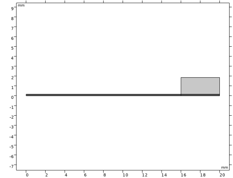
Click to expand the Layers section. In the table, enter the following settings:
|
|
1
|
|
2
|
|
3
|
|
4
|
|
5
|
|
6
|
|
1
|
|
2
|
On the object r1, select Domains 1–3 only.
|
|
3
|
|
4
|
|
5
|
|
6
|
On the object r2, select Boundary 4 only.
|
|
7
|
|
8
|
|
1
|
|
2
|
Go to the Add Material window.
|
|
3
|
|
4
|
Click the Add to Component button in the window toolbar.
|
|
5
|
|
6
|
Click the Add to Component button in the window toolbar.
|
|
7
|
|
1
|
|
2
|
|
3
|
|
1
|
In the Model Builder window, under Component 1 (comp1) > Electrostatics (es) click Charge Conservation, Piezoelectric 1.
|
|
2
|
|
3
|
Click
|
|
4
|
Click
|
|
5
|
|
6
|
Click OK.
|
|
1
|
|
2
|
|
3
|
Click
|
|
4
|
|
5
|
Click OK.
|
|
1
|
|
2
|
|
3
|
Click
|
|
4
|
|
5
|
Click OK.
|
|
6
|
|
7
|
|
1
|
|
2
|
|
3
|
|
4
|
|
1
|
In the Model Builder window, under Component 1 (comp1) > Solid Mechanics (solid) click Piezoelectric Material 1.
|
|
2
|
|
3
|
Click
|
|
4
|
Click
|
|
5
|
|
6
|
Click OK.
|
|
1
|
|
2
|
|
3
|
|
4
|
|
1
|
|
2
|
|
3
|
|
4
|
|
1
|
|
2
|
|
3
|
Click
|
|
4
|
|
5
|
Click OK.
|
|
1
|
|
2
|
Go to the Add Physics window.
|
|
3
|
|
4
|
Click the Add to Component 1 button in the window toolbar.
|
|
5
|
|
1
|
|
2
|
|
4
|
|
1
|
|
2
|
|
3
|
|
4
|
|
1
|
|
2
|
|
3
|
Click
|
|
4
|
|
5
|
Click OK.
|
|
1
|
|
2
|
|
3
|
|
1
|
|
2
|
|
3
|
Click
|
|
4
|
|
5
|
Click OK.
|
|
1
|
|
2
|
|
3
|
|
4
|
Click
|
|
6
|
|
1
|
|
2
|
|
4
|
Click
|
|
6
|
|
1
|
|
2
|
|
3
|
Click
|
|
4
|
|
5
|
Click OK.
|
|
1
|
|
2
|
|
1
|
|
2
|
|
3
|
|
1
|
|
2
|
|
3
|
Clear the Generate default plots checkbox.
|
|
1
|
|
2
|
|
3
|
|
4
|
|
1
|
|
2
|
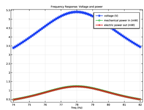
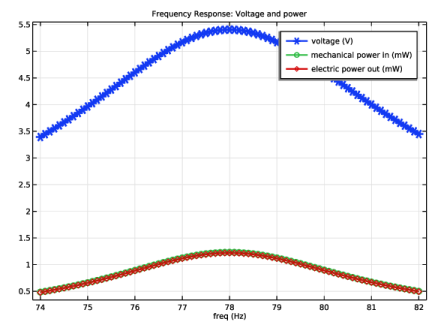
In the Settings window for 1D Plot Group, type Frequency Response: Voltage and Power in the Label text field.
|
|
3
|
|
4
|
|
1
|
|
2
|
|
4
|
|
5
|
|
6
|
|
1
|
|
2
|
Click
|
|
4
|
|
6
|
|
7
|
|
8
|
|
9
|
Click
|
|
11
|
|
12
|
|
13
|
|
14
|
Click
|
|
16
|
|
17
|
|
18
|
|
19
|
|
20
|
|
21
|
|
22
|
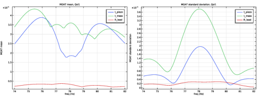
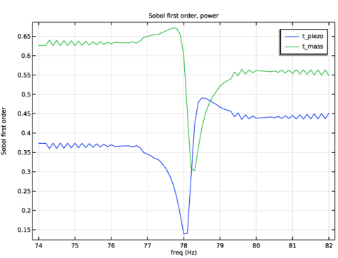
In the Model Builder window, right-click Uncertainty Quantification and choose Add New Uncertainty Quantification Study For > Sensitivity Analysis.
|
|
1
|
|
2
|
In the Settings window for Uncertainty Quantification, locate the Uncertainty Quantification Settings section.
|
|
3
|
|
4
|
Locate the Quantities of Interest section. In the table, enter the following settings:
|
|
5
|
Locate the Input Parameters section. In the table, click to select the cell at row number 3 and column number 1.
|
|
6
|
Click
|
|
7
|
|
8
|
|
9
|
|
10
|
|
11
|
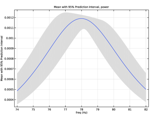
In the Model Builder window, right-click Uncertainty Quantification and choose Add New Uncertainty Quantification Study For > Uncertainty Propagation.
|
|
1
|
|
1
|
In the Model Builder window, under Study 5: Reliability Analysis, EGRA click Uncertainty Quantification.
|
|
2
|
In the Settings window for Uncertainty Quantification, locate the Uncertainty Quantification Settings section.
|
|
3
|
|
4
|
Locate the Quantities of Interest section. In the table, enter the following settings:
|
|
5
|
|
6
|
|
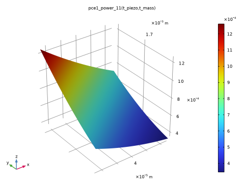
1
|
In the Model Builder window, under Global Definitions click Polynomial Chaos Expansion 1 (pce1_power_1, pce1_power_2, ...).
|
|
2
|
|
3
|
|
4
|