|
|
|
|
1
|
|
2
|
|
3
|
Click Add.
|
|
4
|
Click
|
|
5
|
|
6
|
Click
|
|
1
|
|
2
|
|
3
|
|
1
|
|
2
|
|
1
|
|
2
|
|
1
|
|
2
|
|
1
|
|
2
|
|
3
|
|
4
|
|
5
|
Click
|
|
6
|
|
1
|
|
2
|
On the object sq2, select Point 4 only.
|
|
3
|
|
4
|
|
5
|
Click
|
|
1
|
|
2
|
|
3
|
|
4
|
|
5
|
|
6
|
|
7
|
Click
|
|
1
|
|
2
|
|
3
|
|
4
|
|
5
|
|
6
|
|
7
|
Click
|
|
1
|
In the Model Builder window, under Component 1 (comp1) > Geometry 1 right-click Work Plane 1 (wp1) and choose Extrude.
|
|
2
|
|
4
|
Click
|
|
1
|
|
2
|
|
3
|
|
1
|
|
2
|
Go to the Add Material window.
|
|
3
|
|
4
|
Click the Add to Component button in the window toolbar.
|
|
5
|
|
1
|
|
2
|
|
3
|
Click
|
|
5
|
|
1
|
|
2
|
|
3
|
Click
|
|
5
|
|
1
|
|
3
|
|
1
|
|
1
|
|
3
|
|
4
|
|
1
|
|
3
|
|
4
|
|
1
|
|
3
|
|
4
|
|
1
|
|
2
|
|
1
|
|
2
|
|
1
|
|
2
|
|
3
|
Select the Include geometric nonlinearity checkbox.
|
|
1
|
|
2
|
|
3
|
In the Model Builder window, expand the Study 1 > Solver Configurations > Solution 1 (sol1) > Dependent Variables 1 node, then click Displacement Field (comp1.u).
|
|
4
|
|
5
|
|
6
|
In the Model Builder window, expand the Study 1 > Solver Configurations > Solution 1 (sol1) > Stationary Solver 1 node, then click Fully Coupled 1.
|
|
7
|
|
8
|
|
9
|
|
1
|
|
2
|
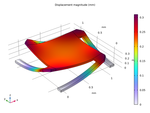
In the Settings window for Volume, click Replace Expression in the upper-right corner of the Expression section. From the menu, choose Component 1 (comp1) > Solid Mechanics > Displacement > solid.disp - Displacement magnitude - m.
|
|
3
|
|
4
|
|
1
|
|
2
|
Go to the Add Material window.
|
|
3
|
|
4
|
Click the Add to Component button in the window toolbar.
|
|
5
|
|
1
|
|
2
|
|
3
|
Select the Auxiliary sweep checkbox.
|
|
4
|
Click
|
|
1
|
|
2
|
|
3
|
In the Model Builder window, expand the Study 1 > Solver Configurations > Solution 2 (sol2) > Dependent Variables 1 node, then click Displacement Field (comp1.u).
|
|
4
|
|
5
|
|
6
|
In the Model Builder window, expand the Study 1 > Solver Configurations > Solution 2 (sol2) > Stationary Solver 1 node, then click Fully Coupled 1.
|
|
7
|
|
8
|
|
9
|
|
1
|
|
2
|
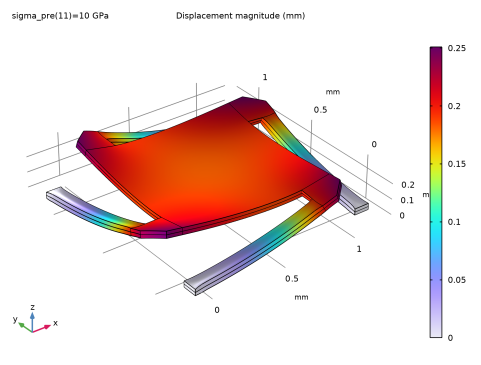
In the Settings window for Volume, click Replace Expression in the upper-right corner of the Expression section. From the menu, choose solid.disp - Displacement magnitude - m.
|
|
3
|
|
4
|
|
1
|
|
2
|
|
3
|
|
4
|
|
5
|
|
6
|
|
1
|
|
2
|
|
3
|
|
4
|
Locate the Plot Settings section.
|
|
5
|
|
1
|
|
2
|
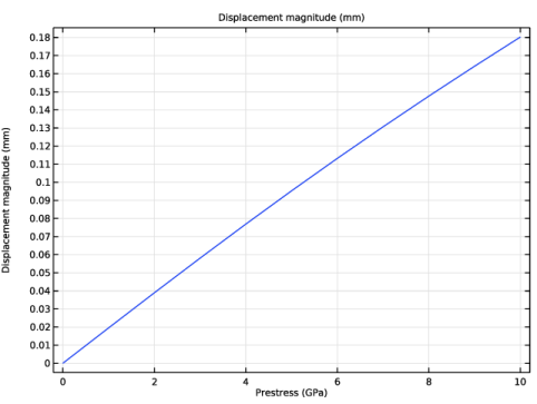
In the Settings window for Point Graph, click Replace Expression in the upper-right corner of the y-Axis Data section. From the menu, choose Component 1 (comp1) > Solid Mechanics > Displacement > solid.disp - Displacement magnitude - m.
|
|
3
|
|
1
|
|
2
|
|
3
|
|
4
|
|
1
|
|
2
|
|
3
|
|
1
|
|
2
|
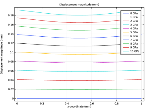
In the Settings window for Line Graph, click Replace Expression in the upper-right corner of the x-Axis Data section. From the menu, choose Component 1 (comp1) > Geometry > Coordinate (spatial frame) > x - x-coordinate.
|
|
3
|
|
4
|