|
|
|
|
•
|
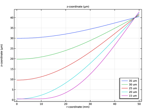
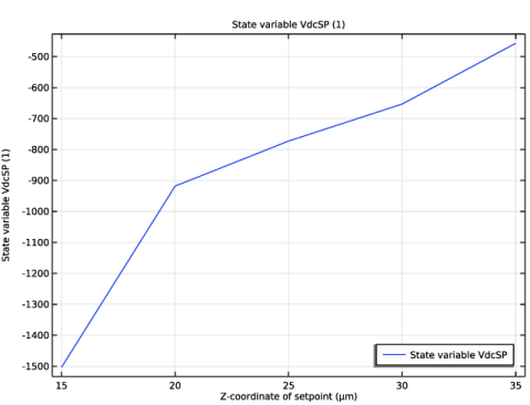
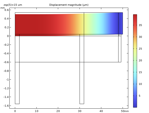
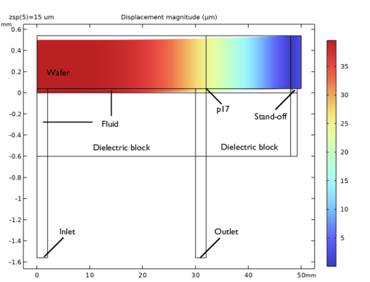
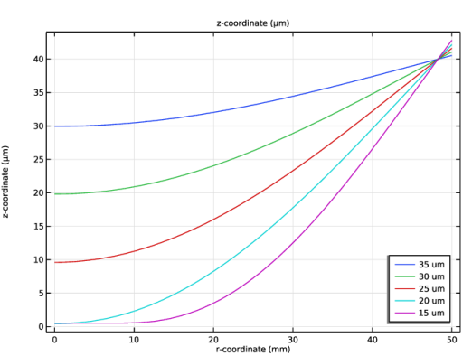
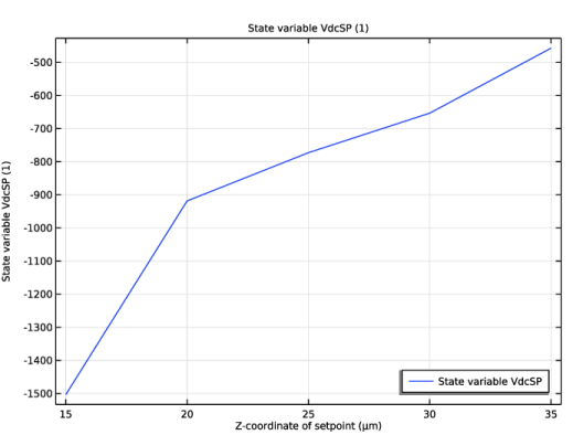
Study 1: Only Solid Mechanics and Electrostatics are enabled to study voltage conditions without gas flow. The study computes the wafer’s profile when zsp is set to 35, 30, 25, 20, and 15 μm. When zsp = 15 μm, the center of the wafer is in contact with the e-chuck.
|
|
•
|
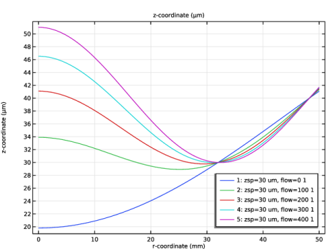
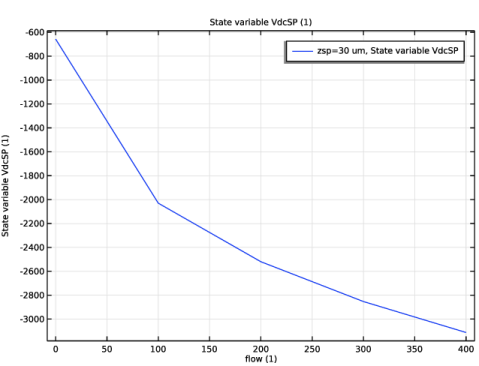
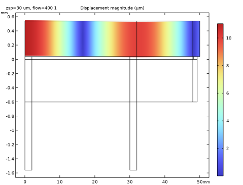
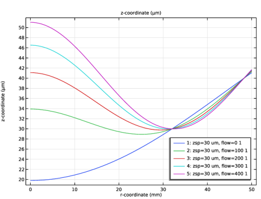
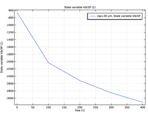
Study 2: The Solid Mechanics, Electrostatics, and Laminar Flow interfaces are enabled to study voltage conditions when the mass flow rate is set to 0, 100, 200, 300, and 400 SCCM and zsp = 30 μm. This study computes the wafer profile and the pressure field within the fluid region.
|
|
•
|
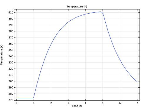
Study 3: In this time-dependent study, all four interfaces, including Heat Transfer, are enabled. This study uses the solution of Study 2 as the initial solution to solve for the temperature field resulting from heat transfer between the e-chuck and the wafer and the plasma process.
|

|
1
|
|
2
|
In the Select Physics tree, select Fluid Flow > Fluid–Structure Interaction > Conjugate Heat Transfer > Fluid–Solid Interaction.
|
|
3
|
Click Add.
|
|
4
|
|
5
|
Click Add.
|
|
6
|
Click
|
|
1
|
|
2
|
|
3
|
|
4
|
Browse to the model’s Application Libraries folder and double-click the file electrostatic_chuck_geometry_parameters.txt.
|
|
1
|
|
2
|
|
3
|
|
4
|
Browse to the model’s Application Libraries folder and double-click the file electrostatic_chuck_mesh_parameters.txt.
|
|
1
|
|
2
|
|
3
|
|
4
|
Browse to the model’s Application Libraries folder and double-click the file electrostatic_chuck_process_parameters.txt.
|
|
1
|
|
2
|
|
3
|
|
4
|
|
1
|
|
2
|
|
1
|
|
2
|
|
3
|
|
1
|
|
2
|
|
3
|
|
4
|
|
5
|
|
6
|
Locate the Selections of Resulting Entities section. Find the Cumulative selection subsection. Click New.
|
|
7
|
|
8
|
Click OK.
|
|
1
|
|
2
|
|
3
|
|
4
|
|
1
|
|
2
|
|
3
|
|
4
|
|
5
|
|
1
|
|
2
|
|
3
|
|
4
|
|
5
|
|
1
|
|
2
|
|
3
|
|
4
|
|
5
|
|
6
|
Locate the Selections of Resulting Entities section. Find the Cumulative selection subsection. Click New.
|
|
7
|
|
8
|
Click OK.
|
|
1
|
In the Model Builder window, expand the Component 1 (comp1) > Definitions > View 1 node, then click Component 1 (comp1) > Geometry 1 > Rectangle 6 (r6).
|
|
2
|
|
3
|
|
4
|
|
5
|
|
6
|
|
7
|
Locate the Selections of Resulting Entities section. Find the Cumulative selection subsection. From the Contribute to list, choose Insulator.
|
|
1
|
|
2
|
|
3
|
Locate the Size and Shape section. In the Width text field, type x_gap3+w_gap3+d_pin-x_outlet-w_outlet.
|
|
4
|
|
5
|
|
6
|
|
7
|
Locate the Selections of Resulting Entities section. Find the Cumulative selection subsection. From the Contribute to list, choose Insulator.
|
|
1
|
|
2
|
|
3
|
|
4
|
|
5
|
|
1
|
|
2
|
|
3
|
|
4
|
|
5
|
|
6
|
|
1
|
|
2
|
|
1
|
|
2
|
|
1
|
|
2
|
|
3
|
|
4
|
|
5
|
|
6
|
|
7
|
On the object uni2, select Boundary 2 only.
|
|
8
|
|
9
|
On the object uni1, select Domain 1 only.
|
|
1
|
|
2
|
On the object pard1, select Domain 6 only.
|
|
3
|
|
4
|
|
5
|
Click in the Graphics window and then press Ctrl+D to clear all objects.
|
|
6
|
|
7
|
On the object uni2, select Boundary 2 only.
|
|
1
|
|
2
|
On the object uni2, select Domain 2 only.
|
|
3
|
|
4
|
|
5
|
|
6
|
On the object pard2, select Boundary 27 only.
|
|
1
|
|
2
|
On the object pard2, select Domain 4 only.
|
|
3
|
|
4
|
|
5
|
|
6
|
On the object pard3, select Boundaries 5 and 8 only.
|
|
1
|
|
2
|
|
3
|
From the Action list, choose Form an assembly. This is necessary because the model includes moving objects.
|
|
4
|
Clear the Create pairs checkbox.
|
|
5
|
Click
|
|
1
|
|
2
|
|
3
|
|
4
|
|
5
|
Click
|
|
1
|
|
2
|
|
3
|
Select the Show geometry labels checkbox.
|
|
1
|
|
2
|
|
3
|
|
4
|
Click
|
|
5
|
|
6
|
Click OK.
|
|
7
|
|
8
|
Clear the Compute integral in revolved geometry checkbox.
|
|
1
|
|
2
|
|
3
|
Click
|
|
4
|
|
5
|
Click OK.
|
|
6
|
|
7
|
Click to select the
|
|
8
|
Click
|
|
9
|
|
10
|
Click OK.
|
|
11
|
|
12
|
|
1
|
|
2
|
|
3
|
Click
|
|
4
|
|
5
|
Click OK.
|
|
6
|
|
7
|
Click to select the
|
|
8
|
Click
|
|
9
|
|
10
|
Click OK.
|
|
11
|
|
12
|
|
1
|
|
2
|
|
3
|
Click
|
|
4
|
|
5
|
Click OK.
|
|
6
|
|
7
|
Click to select the
|
|
8
|
Click
|
|
9
|
|
10
|
Click OK.
|
|
1
|
|
2
|
|
3
|
|
4
|
|
5
|
Click OK.
|
|
1
|
|
2
|
|
3
|
|
4
|
|
5
|
Click OK.
|
|
1
|
|
2
|
|
3
|
Click
|
|
4
|
|
5
|
Click OK.
|
|
6
|
|
7
|
|
1
|
|
1
|
|
2
|
Go to the Add Material window.
|
|
3
|
|
4
|
Click the Add to Component button in the window toolbar.
|
|
1
|
|
2
|
|
1
|
Go to the Add Material window.
|
|
2
|
|
3
|
Click the Add to Component button in the window toolbar.
|
|
1
|
|
2
|
|
1
|
Go to the Add Material window.
|
|
2
|
|
3
|
Click the Add to Component button in the window toolbar.
|
|
4
|
|
1
|
|
2
|
|
3
|
|
1
|
In the Model Builder window, expand the Component 1 (comp1) > Materials > Helium (mat3) > Basic (def) node, then click Piecewise 3 (k).
|
|
2
|
|
3
|
|
4
|
Find the Intervals subsection. In the table, enter the following settings:
|
|
5
|
|
1
|
|
2
|
|
3
|
|
1
|
|
2
|
|
3
|
|
1
|
|
2
|
|
3
|
Select the Disconnect pair checkbox.
|
|
1
|
|
2
|
|
3
|
Click
|
|
4
|
|
5
|
Click OK.
|
|
6
|
|
7
|
From the list, choose Mass flow.
|
|
8
|
|
9
|
|
10
|
|
1
|
|
2
|
|
3
|
Click
|
|
4
|
|
5
|
Click OK.
|
|
6
|
|
7
|
|
8
|
Clear the Suppress backflow checkbox.
|
|
1
|
|
2
|
|
3
|
|
1
|
|
2
|
|
3
|
|
4
|
|
5
|
Click to expand the Contact Surface Offset and Adjustment section. In the doffset,d text field, type 0.5[um].
|
|
6
|
|
7
|
|
8
|
Click OK.
|
|
1
|
|
2
|
|
3
|
|
4
|
|
5
|
Locate the Contact Surface Offset and Adjustment section. Select the Force zero initial gap checkbox.
|
|
1
|
In the Model Builder window, under Component 1 (comp1) click Heat Transfer in Solids and Fluids (ht).
|
|
2
|
|
3
|
|
4
|
Click
|
|
5
|
Click in the Graphics window and then press Ctrl+A to select all domains.
|
|
6
|
|
1
|
In the Model Builder window, under Component 1 (comp1) > Heat Transfer in Solids and Fluids (ht) click Solid 1.
|
|
2
|
|
3
|
|
4
|
|
1
|
|
2
|
|
3
|
|
1
|
|
2
|
|
3
|
|
1
|
|
2
|
|
3
|
|
4
|
|
5
|
Locate the Model Input section. From the Tref list, choose User defined. In the associated text field, type T_chuck.
|
|
6
|
|
1
|
|
2
|
|
3
|
Click
|
|
4
|
|
5
|
Click OK.
|
|
6
|
|
7
|
|
1
|
|
2
|
|
3
|
Click
|
|
4
|
|
5
|
Click OK.
|
|
1
|
|
2
|
|
3
|
Click
|
|
4
|
|
5
|
Click OK.
|
|
6
|
|
7
|
|
1
|
|
2
|
|
3
|
|
4
|
|
1
|
|
2
|
|
3
|
|
1
|
|
2
|
|
3
|
Click
|
|
4
|
|
5
|
Click OK.
|
|
1
|
|
2
|
|
3
|
Click
|
|
4
|
|
5
|
Click OK.
|
|
6
|
|
7
|
|
8
|
|
1
|
|
2
|
|
3
|
Click
|
|
4
|
|
5
|
Click OK.
|
|
6
|
|
7
|
|
8
|
|
9
|
|
10
|
In the Show More Options dialog, in the tree, select the checkbox for the node Physics > Equation Contributions.
|
|
11
|
Click OK.
|
|
1
|
|
2
|
|
1
|
|
2
|
|
3
|
Click
|
|
4
|
|
5
|
Click OK.
|
|
1
|
|
2
|
|
3
|
|
1
|
|
2
|
|
3
|
Click
|
|
4
|
|
5
|
Click OK.
|
|
1
|
|
2
|
|
3
|
|
1
|
|
2
|
|
3
|
Click
|
|
4
|
|
5
|
Click OK.
|
|
1
|
|
2
|
|
3
|
|
4
|
|
5
|
|
6
|
Select the Reverse direction checkbox.
|
|
1
|
|
2
|
|
3
|
Click
|
|
4
|
|
5
|
Click OK.
|
|
1
|
|
2
|
|
3
|
|
4
|
|
5
|
|
6
|
Select the Reverse direction checkbox.
|
|
1
|
|
2
|
|
3
|
|
4
|
Click
|
|
5
|
|
6
|
Click OK.
|
|
1
|
|
2
|
|
3
|
Click
|
|
4
|
|
5
|
Click OK.
|
|
1
|
|
2
|
|
3
|
|
4
|
|
5
|
|
6
|
Select the Symmetric distribution checkbox.
|
|
1
|
|
2
|
|
3
|
|
4
|
Click
|
|
5
|
|
6
|
Click OK.
|
|
7
|
|
1
|
|
2
|
|
3
|
Click
|
|
4
|
|
5
|
Click OK.
|
|
1
|
|
2
|
|
3
|
Click
|
|
4
|
Click
|
|
5
|
|
6
|
Click OK.
|
|
7
|
|
8
|
|
1
|
|
2
|
|
3
|
Click
|
|
4
|
Click
|
|
5
|
|
6
|
Click OK.
|
|
7
|
|
8
|
|
1
|
|
2
|
|
3
|
Click
|
|
4
|
Click
|
|
5
|
|
6
|
Click OK.
|
|
7
|
|
8
|
|
1
|
|
2
|
|
3
|
Click
|
|
4
|
Click
|
|
5
|
|
6
|
Click OK.
|
|
7
|
|
8
|
|
1
|
|
2
|
|
3
|
|
4
|
Click
|
|
5
|
|
6
|
Click OK.
|
|
7
|
|
1
|
|
2
|
|
3
|
|
4
|
Click
|
|
5
|
|
6
|
Click OK.
|
|
1
|
|
2
|
|
3
|
Click
|
|
4
|
|
5
|
Click OK.
|
|
1
|
|
2
|
|
3
|
Click
|
|
4
|
Click
|
|
5
|
|
6
|
Click OK.
|
|
7
|
|
8
|
|
9
|
|
1
|
|
2
|
|
3
|
Click
|
|
4
|
Click
|
|
5
|
|
6
|
Click OK.
|
|
7
|
|
8
|
|
9
|
|
10
|
|
1
|
|
2
|
|
3
|
|
4
|
Click
|
|
5
|
|
6
|
Click OK.
|
|
1
|
|
2
|
|
3
|
Click
|
|
4
|
|
5
|
Click OK.
|
|
1
|
|
2
|
|
3
|
Click
|
|
4
|
Click
|
|
5
|
|
6
|
Click OK.
|
|
7
|
|
8
|
|
9
|
|
10
|
Select the Symmetric distribution checkbox.
|
|
1
|
|
2
|
|
3
|
|
4
|
Click
|
|
5
|
|
6
|
Click OK.
|
|
1
|
|
2
|
|
3
|
Click
|
|
4
|
|
5
|
Click OK.
|
|
1
|
|
2
|
|
3
|
|
1
|
|
3
|
|
4
|
Click to select the
|
|
1
|
|
2
|
|
3
|
|
4
|
Click
|
|
5
|
|
6
|
Click OK.
|
|
1
|
|
2
|
|
3
|
|
4
|
Click
|
|
5
|
|
6
|
Click OK.
|
|
7
|
|
1
|
|
2
|
|
3
|
|
1
|
|
2
|
Go to the Add Study window.
|
|
3
|
|
4
|
Click the Add Study button in the window toolbar.
|
|
5
|
|
1
|
|
2
|
|
1
|
|
2
|
|
3
|
In the Solve for column of the table, under Component 1 (comp1), clear the checkbox for Laminar Flow (spf).
|
|
4
|
In the Solve for column of the table, under Component 1 (comp1), select the checkbox for Solid Mechanics (solid).
|
|
5
|
In the Solve for column of the table, under Component 1 (comp1), clear the checkbox for Heat Transfer in Solids and Fluids (ht).
|
|
6
|
In the Solve for column of the table, under Component 1 (comp1) > Multiphysics, clear the checkboxes for Fluid–Structure Interaction 1 (fsi1), Nonisothermal Flow 1 (nitf1), and Thermal Expansion 1 (te1).
|
|
7
|
Click to expand the Values of Dependent Variables section. Click to expand the Study Extensions section. Select the Auxiliary sweep checkbox.
|
|
8
|
Click
|
|
1
|
|
2
|
|
3
|
In the Model Builder window, expand the Study 1 - Without Gas Flow > Solver Configurations > Solution 1 (sol1) > Stationary Solver 1 node.
|
|
4
|
Right-click Study 1 - Without Gas Flow > Solver Configurations > Solution 1 (sol1) > Stationary Solver 1 and choose Fully Coupled.
|
|
5
|
|
6
|
|
7
|
|
8
|
|
1
|
|
2
|
Go to the Add Study window.
|
|
3
|
|
4
|
Click the Add Study button in the window toolbar.
|
|
5
|
|
1
|
|
2
|
|
1
|
|
2
|
|
3
|
In the Solve for column of the table, under Component 1 (comp1), clear the checkbox for Heat Transfer in Solids and Fluids (ht).
|
|
4
|
In the Solve for column of the table, under Component 1 (comp1) > Multiphysics, clear the checkbox for Thermal Expansion 1 (te1).
|
|
5
|
Click to expand the Values of Dependent Variables section. Find the Initial values of variables solved for subsection. From the Settings list, choose User controlled.
|
|
6
|
|
7
|
|
8
|
|
9
|
|
10
|
|
11
|
Click
|
|
13
|
Click
|
|
1
|
|
2
|
|
3
|
In the Model Builder window, expand the Study 2 - With Gas Flow > Solver Configurations > Solution 2 (sol2) > Stationary Solver 1 node.
|
|
4
|
Right-click Study 2 - With Gas Flow > Solver Configurations > Solution 2 (sol2) > Stationary Solver 1 and choose Fully Coupled.
|
|
5
|
|
1
|
|
2
|
Go to the Add Study window.
|
|
3
|
|
4
|
Click the Add Study button in the window toolbar.
|
|
5
|
|
1
|
In the Settings window for Study, type Study 3 - Wafer Temperature vs. Time in the Label text field.
|
|
2
|
|
1
|
In the Model Builder window, under Study 3 - Wafer Temperature vs. Time click Step 1: Time Dependent.
|
|
2
|
|
3
|
In the Solve for column of the table, under Component 1 (comp1) > Multiphysics, clear the checkbox for Thermal Expansion 1 (te1).
|
|
4
|
|
5
|
|
6
|
Click to expand the Values of Dependent Variables section. Find the Initial values of variables solved for subsection. From the Settings list, choose User controlled.
|
|
7
|
|
8
|
|
9
|
|
10
|
|
11
|
Click
|
|
13
|
Click
|
|
15
|
Click
|
|
1
|
|
2
|
|
3
|
In the Model Builder window, expand the Study 3 - Wafer Temperature vs. Time > Solver Configurations > Solution 3 (sol3) > Time-Dependent Solver 1 node.
|
|
4
|
Right-click Study 3 - Wafer Temperature vs. Time > Solver Configurations > Solution 3 (sol3) > Time-Dependent Solver 1 and choose Fully Coupled.
|
|
5
|
|
6
|
|
7
|
Click to expand the Method and Termination section. From the Nonlinear method list, choose Automatic highly nonlinear (Newton).
|
|
8
|
|
9
|
|
1
|
|
2
|
In the Settings window for 1D Plot Group, type Wafer Profile, Without Gas Flow in the Label text field.
|
|
1
|
|
2
|
|
3
|
Click
|
|
4
|
|
5
|
Click OK.
|
|
6
|
|
7
|
|
8
|
|
9
|
Select the Description checkbox.
|
|
10
|
|
11
|
|
12
|
|
1
|
|
2
|
|
3
|
|
4
|
|
1
|
|
2
|
|
1
|
|
2
|
|
4
|
|
5
|
|
6
|
|
7
|
Select the Description checkbox.
|
|
8
|
|
1
|
|
2
|
|
3
|
In the Settings window for 1D Plot Group, type Wafer Profile, With Gas Flow in the Label text field.
|
|
4
|
|
5
|
|
6
|
Click
|
|
1
|
|
2
|
|
3
|
|
4
|
|
1
|
|
2
|
|
3
|
|
1
|
|
2
|
|
3
|
|
4
|
|
5
|
|
1
|
|
2
|
|
3
|
|
4
|
|
1
|
|
2
|
In the Settings window for 2D Plot Group, type Displacement, Without Gas Flow in the Label text field.
|
|
1
|
|
2
|
|
3
|
|
4
|
|
5
|
Select the Description checkbox.
|
|
6
|
|
1
|
|
2
|
|
3
|
|
4
|
|
5
|
|
1
|
|
2
|
|
3
|
|
1
|
|
2
|
|
3
|
|
4
|
|
5
|
Select the Description checkbox.
|
|
6
|
|
1
|
|
2
|
|
3
|
Select the Description checkbox.
|
|
4
|
Locate the Scale section.
|
|
5
|
|
6
|
|
7
|
|
1
|
|
2
|
|
3
|
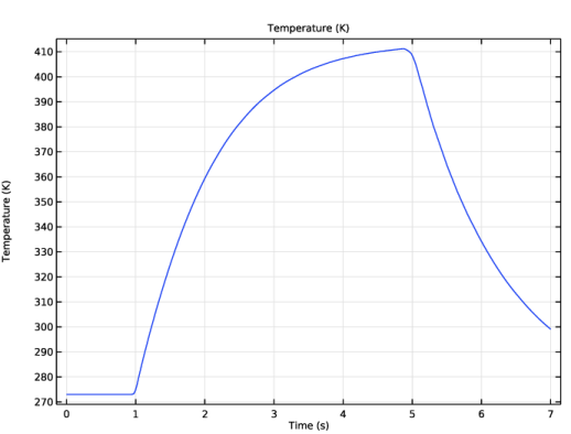
Locate the Data section. From the Dataset list, choose Study 3 - Wafer Temperature vs. Time/Solution 3 (sol3).
|
|
1
|
|
3
|
|
4
|
|
5
|
Select the Description checkbox.
|
|
6
|
|
7
|