
PDF

Birdbath Resonator Gyroscope
Introduction
This tutorial shows how to model and analyze a birdbath resonator gyroscope (BRG), a type of Coriolis vibratory gyroscope invented at the University of Michigan and commercialized by Enertia Microsystems as a millimeter-scale navigation-grade gyroscope. This tutorial shows how the gyroscope’s axisymmetric shape allows coupling between drive and sense modes and how the Coriolis force is measured.
Used in an inertial measurement unit (IMU), a gyroscope provides information on its position and orientation for navigation. A BRG has an axisymmetric structure made of fused quartz that gives it high sensitivity and high quality factor. A BRG can be much more accurate than commercial MEMS gyroscopes and match the performance of larger and more expensive gyroscopes. The BRG design minimizes cost, weight, size, and power consumption while delivering higher accuracy and stability. Based on Ref. 1, the model in this tutorial demonstrates the principles of BRG operation.
Model Definition
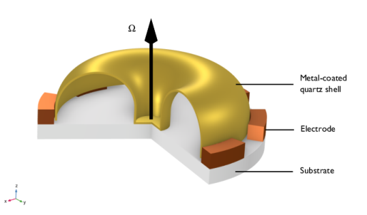
Figure 1 shows a cut-away diagram of a typical BRG (not of the actual model) comprising a conductive fused-quartz shell, four pairs of electrodes, and a substrate. The center of the shell is anchored to the substrate whereas its outer rim is free. The electrodes are positioned around it, forming parallel plate capacitors with small gaps. In this model, two electrodes are used to drive the gyroscope; one is used for sensing and the remaining are grounded. FEM can be used to compute the shell’s deformation and frequency response under the effects of the Coriolis force due to the angular velocity Ω.
Figure 1: Cut-away diagram of a typical BRG comprising metal-coated quartz shell, electrodes, and substrate. The angular velocity of the rotating frame is Ω, as indicated by the arrow through the center of the BRG.
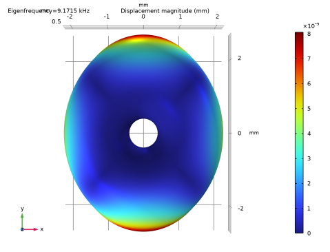
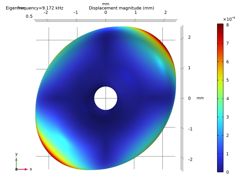
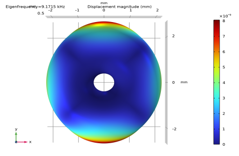
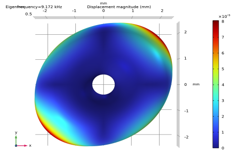
Due to the axisymmetry of the shell, this type of gyroscopes has two eigenmodes with nearly identical frequencies oriented 45° apart. These so-called n = 2 wine-glass modes are shown in Figure 2. Typically, the positions of drive and sense electrodes are aligned with the lower and the higher frequency modes, respectively. However, the higher frequency is applied to the drive electrodes to facilitate excitation of the second mode under Coriolis force. Its sensitivity to the Coriolis force arises from how easily the two modes can become coupled.
As the drive mode vibrates within the rotating frame, the Coriolis body force acts on the structure which excites the sense mode. The Coriolis force (Fcor) is given by
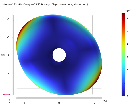
where ρ is the density of the material, Ω is the angular velocity of the rotating frame, and u is the local displacement of the structure. From the above equation, it is clear that the Coriolis force is maximal when the angular velocity of the frame is parallel to the symmetry axis of the shell. In this case, the resulting force is in the in plane direction and produces a corresponding in-plane motion. This motion causes reaction moments along the rim of the shell, thereby exciting the sense mode. The sense electrodes measure the floating potential, converting the motion to electrical signal with a characteristic waveform.
Figure 2: The two mode shapes of the BRG have nearly identical frequencies and are oriented 45° apart.
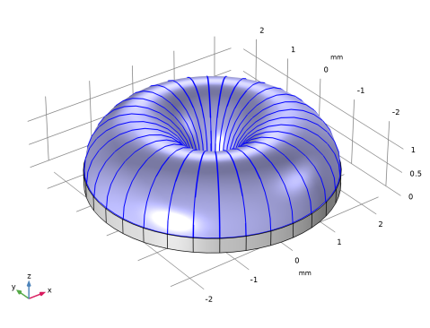
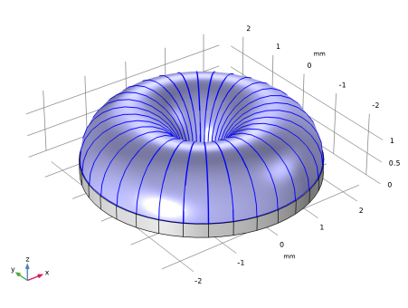
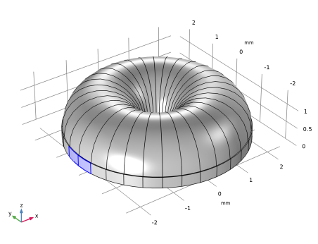
Rather than modeling the 30 μm-thick shell as a 3D volume, here you model the vibrating structure as a Linear Elastic Material shell under the Shell interface (requires a Structural Mechanics Module license) as shown in Figure 3. For convenience, create the geometry and the mesh based on an 11.25° sector. The shell is defined as a perfect conductor with mechanical properties of fused quartz. In a real device, the shell could be made of fused quartz and coated with metal such as gold or platinum. Use the SiO2 material model from the MEMS material library because it most closely matches the mechanical properties of fused quartz.
Figure 3: The shell domain of the BRG modeled using the Shell interface (requiring a Structural Mechanics Module license).
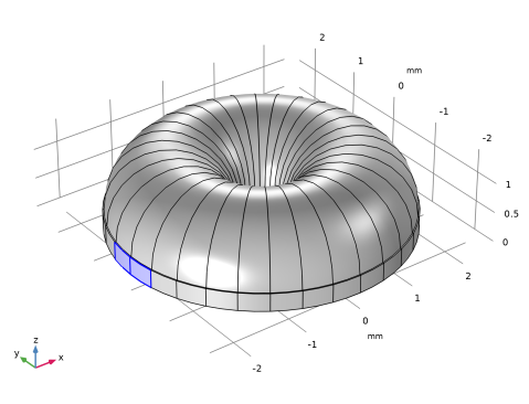
The shell and the electrodes form parallel-plate capacitors with 20 μm gaps which are very small relative to their areas so edge effects can be neglected to simplify geometry and mesh creation. Use Boundary Terminal features to represent the electrode surfaces opposite of the shell rather than model the electrodes as 3D objects. To minimize the size of the model, do not include the free space around the gyroscope and specify the electrostatics domain as a 20 μm-thick ring between the shell and the terminals. Set a 25 V potential difference with 1 V harmonic perturbation between the shell and drive electrodes. As previously mentioned, the drive electrodes are aligned with the lower-frequency mode shape, as seen in Figure 4.
Figure 4: The electrostatic domain comprising terminal boundaries, the opposing surface of the shell, and a 20 um gap between them.
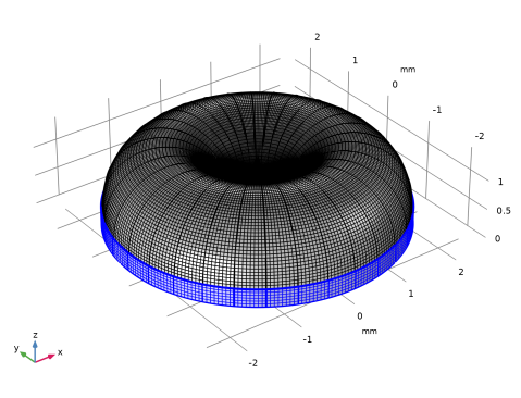
Rotation is modeled using the Rotating Frame feature of the Shell interface with the Coriolis force and Spin softening features enabled. In general, resonant structures require a very fine mesh to achieve an accurate frequency response. To save time, use a relatively coarse mesh for this tutorial and anticipate resonant peaks to shift if a finer mesh is used instead. The mesh is parameterized as a preparation for refinement studies. Follow the detailed steps in the Modeling Instructions section below.
Results and Discussion
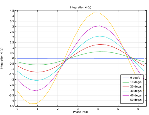
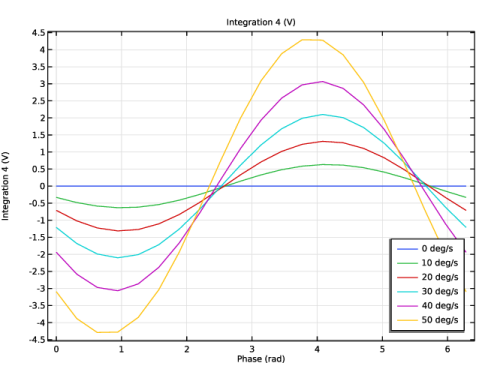
Figure 2 above shows the n = 2 wine glass eigenmodes computed with a Prestressed Eigenfrequency study. Based on this result, use the higher frequency in the subsequent Frequency Domain Perturbation study to analyze the effect of angular velocity on the gyroscope. Figure 5 shows the plots of voltage versus phase measured by the sense (floating) electrode for Ω = 0, 10, 20, 30, 40 and 50 rad/s. This result shows how the angular velocity can be read by an electronic circuit that measures and amplifies the voltage at the floating electrodes as a signal with an amplitude that is proportional to the Coriolis force.
Note that a real BRG can be connected to a complex control loop that generates a signal to negate the effect of Coriolis force. In this mode of operation, the amplitude and phase of this control signal become the measure of the Coriolis force.
Figure 5: Floating potential measured at the sense electrode as a function of phase for angular velocities 0, 10, 20, 30, 40 and 50 rad/s.
Reference
1. J.Y. Cho and others, “1.5-Million Q-Factor Vacuum-Packaged Birdbath Resonator Gyroscope (BRG),” 2019 IEEE 32nd International Conference on Micro Electro Mechanical Systems (MEMS), Seoul, Korea (South), pp. 210–213, 2019.
Application Library path: MEMS_Module/Sensors/birdbath_resonator_gyroscope
Modeling Instructions
From the File menu, choose New.
New
In the New window, click  Model Wizard.
Model Wizard
1
In the Model Wizard window, Start by creating a new 3D model with an Electromechanics, Shell multiphysics interface.
2
3
In the Select Physics tree, select AC/DC > Electromagnetics and Mechanics > Electromechanics > Electromechanics, Shell.
4
Click Add.
5
Click  Study.
6
In the Select Study tree, select Preset Studies for Selected Physics Interfaces > Shell > Eigenfrequency, Prestressed.
7
Geometry 1
The Model Wizard starts the COMSOL Desktop at the Geometry node. Take the opportunity to set the length unit to millimeter for convenience.
1
In the Model Builder window, under Component 1 (comp1) click Geometry 1.
2
In the Settings window for Geometry, locate the Units section.
3
From the Length unit list, choose mm.
Define and specify the parameters of the model.
Global Definitions
Parameters 1
1
In the Model Builder window, under Global Definitions click Parameters 1.
2
In the Settings window for Parameters, locate the Parameters section.
3
Geometry 1
Work Plane 1 (wp1)
1
In the Geometry toolbar, click  Work Plane.
2
In the Settings window for Work Plane, locate the Plane Definition section.
3
From the Plane list, choose xz-plane.
Work Plane 1 (wp1) > Plane Geometry
In the Model Builder window, click Plane Geometry.
Work Plane 1 (wp1) > Circular Arc 1 (ca1)
1
In the Work Plane toolbar, click  More Primitives and choose Circular Arc.
2
In the Settings window for Circular Arc, locate the Center section.
3
In the xw text field, type r+rc.
4
In the yw text field, type ha.
5
Locate the Radius section. In the Radius text field, type r.
6
Locate the Angles section. In the End angle text field, type 180.
Work Plane 1 (wp1) > Line Segment 1 (ls1)
1
In the Work Plane toolbar, click  More Primitives and choose Line Segment.
2
On the object ca1, select Point 2 only.
3
In the Settings window for Line Segment, locate the Endpoint section.
4
From the Specify list, choose Coordinates.
5
In the xw text field, type rc.
Work Plane 1 (wp1) > Rectangle 1 (r1)
1
In the Work Plane toolbar, click  Rectangle.
2
In the Settings window for Rectangle, locate the Size and Shape section.
3
In the Width text field, type d.
4
In the Height text field, type he.
5
Locate the Position section. In the xw text field, type rc+2*r.
6
In the yw text field, type ha-he.
7
Click  Build Selected.
Revolve 1 (rev1)
1
In the Model Builder window, under Component 1 (comp1) > Geometry 1 right-click Work Plane 1 (wp1) and choose Revolve.
2
In the Settings window for Revolve, locate the Revolution Angles section.
3
Click the Angles button.
4
In the Start angle text field, type 78.75.
5
In the End angle text field, type 90.
6
Click  Build Selected.
Rotate 1 (rot1)
1
In the Geometry toolbar, click  Transforms and choose Rotate.
2
3
In the Settings window for Rotate, locate the Input section.
4
Select the Keep input objects checkbox.
5
Locate the Rotation section. Click  Range.
6
In the Range dialog, type 11.25 in the Start text field.
7
In the Step text field, type 11.25.
8
In the Stop text field, type 348.75.
9
Click Replace.
10
In the Settings window for Rotate, click  Build Selected.
11
Click  Build Selected.
Define selections for the electrodes and other boundaries and domains to make specifying material models and physics interface features easier.
Definitions
Gap
1
In the Definitions toolbar, click  Box.
2
In the Settings window for Box, type Gap in the Label text field.
Shell
1
In the Definitions toolbar, click  Cylinder.
2
In the Settings window for Cylinder, type Shell in the Label text field.
3
Locate the Geometric Entity Level section. From the Level list, choose Boundary.
4
Locate the Size and Shape section. In the Outer radius text field, type rc+2*r+0.01.
5
Locate the Output Entities section. From the Include entity if list, choose Entity inside cylinder.
Drive
1
In the Definitions toolbar, click  Explicit.
2
In the Settings window for Explicit, type Drive in the Label text field.
3
Locate the Input Entities section. From the Geometric entity level list, choose Boundary.
4
Click  Paste Selection.
5
In the Paste Selection dialog, type 2 3 222 223 in the Selection text field.
6
Sense
1
In the Definitions toolbar, click  Explicit.
2
In the Settings window for Explicit, type Sense in the Label text field.
3
Locate the Input Entities section. From the Geometric entity level list, choose Boundary.
4
Click  Paste Selection.
5
In the Paste Selection dialog, type 182 192 in the Selection text field.
6
Ground
1
In the Definitions toolbar, click  Explicit.
2
In the Settings window for Explicit, type Ground in the Label text field.
3
Locate the Input Entities section. From the Geometric entity level list, choose Boundary.
4
Click  Paste Selection.
5
In the Paste Selection dialog, type 37, 41, 49, 53, 85, 89, 113, 125, 183, 193 in the Selection text field.
6
Fixed Boundary
1
In the Definitions toolbar, click  Box.
2
In the Settings window for Box, type Fixed Boundary in the Label text field.
3
Locate the Geometric Entity Level section. From the Level list, choose Edge.
4
Locate the Box Limits section. In the z maximum text field, type 0.01.
5
Locate the Output Entities section. From the Include entity if list, choose Entity inside box.
Roller Bottom
1
Right-click Fixed Boundary and choose Duplicate.
2
In the Settings window for Box, type Roller Bottom in the Label text field.
3
Locate the Geometric Entity Level section. From the Level list, choose Boundary.
4
Locate the Box Limits section. In the z maximum text field, type ha-he+0.001.
Roller Top
1
Right-click Roller Bottom and choose Duplicate.
2
In the Settings window for Box, type Roller Top in the Label text field.
3
Locate the Box Limits section. In the z minimum text field, type ha-0.001.
4
In the z maximum text field, type ha+0.001.
Roller Side
1
In the Definitions toolbar, click  Explicit.
2
In the Settings window for Explicit, type Roller Side in the Label text field.
3
Locate the Input Entities section. From the Geometric entity level list, choose Boundary.
4
Click  Paste Selection.
5
In the Paste Selection dialog, type 12, 16, 36, 40, 60, 64, 84, 88, 154, 158, 174, 178, 194, 198, 214, 218 in the Selection text field.
6
Add SiO2 material to the model and specify the regions it belongs to.
Add Material
1
In the Materials toolbar, click  Add Material to open the Add Material window.
2
Go to the Add Material window.
3
In the tree, select MEMS > Insulators > SiO2 - Silicon oxide.
4
Click the Add to Component button in the window toolbar.
5
In the Materials toolbar, click  Add Material to close the Add Material window.
Materials
SiO2 - Silicon oxide (mat1)
1
In the Settings window for Material, locate the Geometric Entity Selection section.
2
From the Geometric entity level list, choose Boundary.
3
From the Selection list, choose Shell.
Moving Mesh
Deforming Domain 1
1
In the Model Builder window, under Component 1 (comp1) > Moving Mesh click Deforming Domain 1.
2
In the Settings window for Deforming Domain, locate the Domain Selection section.
3
From the Selection list, choose Gap.
Symmetry/Roller 1
1
In the Model Builder window, click Symmetry/Roller 1.
2
In the Settings window for Symmetry/Roller, locate the Boundary Selection section.
3
From the Selection list, choose Roller Top.
Symmetry/Roller 2
1
Right-click Component 1 (comp1) > Moving Mesh > Symmetry/Roller 1 and choose Duplicate.
2
In the Settings window for Symmetry/Roller, locate the Boundary Selection section.
3
From the Selection list, choose Roller Bottom.
Symmetry/Roller 3
Right-click Symmetry/Roller 2 and choose Duplicate.
Symmetry/Roller 2
From the Selection list, choose Roller Side.
Specify the settings for the Electrostatics interface.
Electrostatics (es)
Shell
1
In the Physics toolbar, click  Boundaries and choose Boundary Terminal.
2
In the Settings window for Boundary Terminal, type Shell in the Label text field.
3
Locate the Boundary Selection section. From the Selection list, choose Shell.
4
Locate the Terminal section. From the Terminal type list, choose Voltage.
5
In the V0 text field, type Vdc.
Drive electrodes
1
Right-click Shell and choose Duplicate.
2
In the Settings window for Boundary Terminal, type Drive electrodes in the Label text field.
3
Locate the Boundary Selection section. From the Selection list, choose Drive.
4
Locate the Terminal section. In the V0 text field, type 0.
Harmonic Perturbation 1
1
In the Physics toolbar, click  Attributes and choose Harmonic Perturbation.
2
In the Settings window for Harmonic Perturbation, locate the Terminal section.
3
In the V0 text field, type Vdrive.
Ground 1
1
In the Physics toolbar, click  Boundaries and choose Ground.
2
In the Settings window for Ground, locate the Boundary Selection section.
3
From the Selection list, choose Ground.
Sense electrode
1
In the Physics toolbar, click  Boundaries and choose Floating Potential.
2
In the Settings window for Floating Potential, type Sense electrode in the Label text field.
3
Locate the Boundary Selection section. From the Selection list, choose Sense.
Define some integration operators for results processing.
Definitions
Integration 1 (intop1)
1
In the Definitions toolbar, click  Nonlocal Couplings and choose Integration.
2
In the Settings window for Integration, locate the Source Selection section.
3
From the Geometric entity level list, choose Point.
4
Integration 2 (intop2)
1
In the Definitions toolbar, click  Nonlocal Couplings and choose Integration.
2
In the Settings window for Integration, locate the Source Selection section.
3
From the Geometric entity level list, choose Point.
4
Integration 3 (intop3)
1
In the Definitions toolbar, click  Nonlocal Couplings and choose Integration.
2
In the Settings window for Integration, locate the Source Selection section.
3
From the Geometric entity level list, choose Point.
4
Integration 4 (intop4)
1
In the Definitions toolbar, click  Nonlocal Couplings and choose Integration.
2
In the Settings window for Integration, locate the Source Selection section.
3
From the Geometric entity level list, choose Point.
4
Specify the settings for the Shell interface.
Shell (shell)
1
In the Model Builder window, under Component 1 (comp1) click Shell (shell).
2
In the Settings window for Shell, locate the Boundary Selection section.
3
From the Selection list, choose Shell.
Linear Elastic Material 1
In the Model Builder window, under Component 1 (comp1) > Shell (shell) click Linear Elastic Material 1.
Damping 1
1
In the Physics toolbar, click  Attributes and choose Damping.
2
In the Settings window for Damping, locate the Damping Settings section.
3
From the Damping type list, choose Isotropic loss factor.
4
From the ηs list, choose User defined. In the associated text field, type 1/Q.
Thickness and Offset 1
1
In the Model Builder window, under Component 1 (comp1) > Shell (shell) click Thickness and Offset 1.
2
In the Settings window for Thickness and Offset, locate the Thickness and Offset section.
3
In the d0 text field, type ts.
4
From the Position list, choose Top surface on boundary.
Rotating Frame 1
1
In the Physics toolbar, click  Boundaries and choose Rotating Frame.
2
In the Settings window for Rotating Frame, locate the Rotating Frame section.
3
In the ωr text field, type Omega.
4
Locate the Frame Acceleration Effect section. Select the Coriolis force checkbox.
Fixed Constraint 1
1
In the Physics toolbar, click  Edges and choose Fixed Constraint.
2
In the Settings window for Fixed Constraint, locate the Edge Selection section.
3
From the Selection list, choose Fixed Boundary.
Create the mesh for the model.
Mesh 1
Click the  Wireframe Rendering button in the Graphics toolbar.
Edge 1
1
In the Mesh toolbar, click  More Generators and choose Edge.
2
In the Settings window for Edge, locate the Edge Selection section.
3
Click  Paste Selection.
4
In the Paste Selection dialog, type 203 205 207 274 in the Selection text field.
5
Distribution 1
1
Right-click Edge 1 and choose Distribution.
2
In the Settings window for Distribution, locate the Edge Selection section.
3
4
Click  Remove from Selection.
5
6
7
Click  Remove from Selection.
8
9
Locate the Distribution section. In the Number of elements text field, type 8.
Distribution 2
1
In the Model Builder window, right-click Edge 1 and choose Distribution.
2
In the Settings window for Distribution, locate the Edge Selection section.
3
4
Click  Remove from Selection.
5
6
7
Click  Remove from Selection.
8
9
Locate the Distribution section. In the Number of elements text field, type 6.
Mapped 1
1
In the Mesh toolbar, click  More Generators and choose Mapped.
2
In the Settings window for Mapped, locate the Boundary Selection section.
3
Click  Paste Selection.
4
In the Paste Selection dialog, type 122 in the Selection text field.
5
Edge 2
1
In the Mesh toolbar, click  More Generators and choose Edge.
2
In the Settings window for Edge, locate the Edge Selection section.
3
Click  Paste Selection.
4
In the Paste Selection dialog, type 199-202, 215, 218 in the Selection text field.
5
Distribution 1
1
Right-click Edge 2 and choose Distribution.
2
In the Settings window for Distribution, locate the Edge Selection section.
3
4
Click  Remove from Selection.
5
6
7
Click  Remove from Selection.
8
9
Locate the Distribution section. In the Number of elements text field, type 60.
Distribution 2
1
In the Model Builder window, right-click Edge 2 and choose Distribution.
2
In the Settings window for Distribution, locate the Edge Selection section.
3
4
Click  Remove from Selection.
5
6
7
Click  Remove from Selection.
8
9
Locate the Distribution section. In the Number of elements text field, type 8.
Mapped 2
1
In the Mesh toolbar, click  More Generators and choose Mapped.
2
Swept 1
1
In the Mesh toolbar, click  Swept.
2
In the Settings window for Swept, locate the Domain Selection section.
3
From the Geometric entity level list, choose Domain.
4
5
Click to expand the Source Faces section. Click  Paste Selection.
6
In the Paste Selection dialog, type 122 in the Selection text field.
7
8
In the Settings window for Swept, click to expand the Destination Faces section.
9
Click  Paste Selection.
10
In the Paste Selection dialog, type 125 in the Selection text field.
11
Distribution 1
1
Right-click Swept 1 and choose Distribution.
2
In the Settings window for Distribution, locate the Distribution section.
3
In the Number of elements text field, type 4.
4
Click  Build Selected.
Copy Face 1
1
In the Mesh toolbar, click  Copy and choose Copy Face.
2
In the Settings window for Copy Face, locate the Source Boundaries section.
3
Click  Paste Selection.
4
In the Paste Selection dialog, type 120 in the Selection text field.
5
6
In the Settings window for Copy Face, locate the Destination Boundaries section.
7
Click  Paste Selection.
8
In the Paste Selection dialog, type 10, 11, 21, 23, 33, 35, 45, 47, 57, 59, 69, 71, 81, 83, 93, 95, 117, 127, 129, 131, 133, 135, 137, 139, 141, 143, 145, 147, 149, 151, 153 in the Selection text field.
9
Copy Face 2
1
In the Mesh toolbar, click  Copy and choose Copy Face.
2
In the Settings window for Copy Face, locate the Source Boundaries section.
3
Click  Paste Selection.
4
In the Paste Selection dialog, type 119 in the Selection text field.
5
6
In the Settings window for Copy Face, locate the Destination Boundaries section.
7
Click  Paste Selection.
8
In the Paste Selection dialog, type 96-111, 118, 126, 128, 130, 132, 134, 136, 138, 140, 142, 144, 146, 148, 150, 152 in the Selection text field.
9
10
In the Settings window for Copy Face, click  Build Selected.
Copy 1
1
In the Mesh toolbar, click  Copy and choose Copy.
2
In the Settings window for Copy, locate the Dimension section.
3
From the Geometric entity level list, choose Domain.
4
Locate the Source Entities section. Click  Paste Selection.
5
In the Paste Selection dialog, type 18 in the Selection text field.
6
7
In the Settings window for Copy, locate the Destination Entities section.
8
Click to select the  Activate Selection toggle button.
9
Click  Paste Selection.
10
In the Paste Selection dialog, type 1-17, 19-32 in the Selection text field.
11
12
In the Settings window for Copy, click  Build Selected.
Set up and compute the Prestressed Eigenfrequency study.
Study 1 - Prestressed Eigenfrequency
1
In the Model Builder window, click Study 1.
2
In the Settings window for Study, type Study 1 - Prestressed Eigenfrequency in the Label text field.
3
Locate the Study Settings section. Clear the Generate default plots checkbox.
Step 2: Eigenfrequency
1
In the Model Builder window, under Study 1 - Prestressed Eigenfrequency click Step 2: Eigenfrequency.
2
In the Settings window for Eigenfrequency, locate the Study Settings section.
3
From the Unit list, choose kHz.
4
In the Search for eigenfrequencies around shift text field, type 1.
For the study to solve, disable the Floating Potential boundary.
5
Locate the Physics and Variables Selection section. Select the Modify model configuration for study step checkbox.
6
In the tree, select Component 1 (comp1) > Electrostatics (es) > Sense electrode.
7
8
In the Study toolbar, click  Compute.
Set up a Frequency Domain Perturbation study using the sense mode frequency from the previous study.
Add Study
1
In the Study toolbar, click  Add Study to open the Add Study window.
2
Go to the Add Study window.
3
Find the Studies subsection. In the Select Study tree, select Preset Studies for Selected Physics Interfaces > Shell > Frequency Domain, Prestressed.
4
Click the Add Study button in the window toolbar.
5
In the Study toolbar, click  Add Study to close the Add Study window.
Study 2 - Frequency Domain Perturbation
1
In the Settings window for Study, type Study 2 - Frequency Domain Perturbation in the Label text field.
2
Locate the Study Settings section. Clear the Generate default plots checkbox.
Step 2: Frequency-Domain Perturbation
1
In the Model Builder window, under Study 2 - Frequency Domain Perturbation click Step 2: Frequency-Domain Perturbation.
2
In the Settings window for Frequency-Domain Perturbation, locate the Study Settings section.
3
From the Frequency unit list, choose kHz.
4
In the Frequencies text field, type 9.172.
5
Click to expand the Study Extensions section. Select the Auxiliary sweep checkbox.
6
7
8
In the Study toolbar, click  Compute.
Results
Create plot to show the shapes of the eigenmodes.
Mode Shape
1
In the Results toolbar, click  3D Plot Group.
2
In the Settings window for 3D Plot Group, type Mode Shape in the Label text field.
3
Locate the Plot Settings section. Clear the Plot dataset edges checkbox.
Surface 1
1
Right-click Mode Shape and choose Surface.
2
In the Settings window for Surface, click Replace Expression in the upper-right corner of the Expression section. From the menu, choose Component 1 (comp1) > Shell > Displacement > shell.disp - Displacement magnitude - m.
3
Locate the Expression section. Select the Description checkbox.
Deformation 1
1
Right-click Surface 1 and choose Deformation.
2
Click the  Zoom Extents button in the Graphics toolbar.
3
Click the  Go to XY View button in the Graphics toolbar.
Surface 1
1
In the Model Builder window, click Surface 1.
2
In the Settings window for Surface, click  Plot Next.
Create plot to show the displacement from the frequency domain study.
Displacement
1
In the Results toolbar, click  3D Plot Group.
2
In the Settings window for 3D Plot Group, type Displacement in the Label text field.
3
Locate the Data section. From the Dataset list, choose Study 2 - Frequency Domain Perturbation/Solution 3 (sol3).
4
Locate the Plot Settings section. Clear the Plot dataset edges checkbox.
Surface 1
1
Right-click Displacement and choose Surface.
2
In the Settings window for Surface, click Replace Expression in the upper-right corner of the Expression section. From the menu, choose Component 1 (comp1) > Shell > Displacement > shell.disp - Displacement magnitude - m.
3
Locate the Expression section. Select the Description checkbox.
Deformation 1
1
Right-click Surface 1 and choose Deformation.
2
Click the  Zoom Extents button in the Graphics toolbar.
3
Click the  Go to XY View button in the Graphics toolbar.
Create a 1D plot of potential at the sense terminal as a function of phase.
Sense Electrode Potential
1
In the Results toolbar, click  1D Plot Group.
2
In the Settings window for 1D Plot Group, locate the Data section.
3
From the Dataset list, choose Study 2 - Frequency Domain Perturbation/Solution 3 (sol3).
4
In the Label text field, type Sense Electrode Potential.
Global 1
1
Right-click Sense Electrode Potential and choose Global.
2
In the Settings window for Global, locate the y-Axis Data section.
3
4
Locate the x-Axis Data section. From the Parameter list, choose Phase.
5
Click to expand the Legends section. From the Legends list, choose Automatic.
6
Find the Include subsection. Clear the Description checkbox.
7
In the Sense Electrode Potential toolbar, click  Plot.
8
From the Legends list, choose Manual.
9
Sense Electrode Potential
1
In the Model Builder window, click Sense Electrode Potential.
2
In the Settings window for 1D Plot Group, locate the Legend section.
3
From the Position list, choose Lower right.
4
In the Sense Electrode Potential toolbar, click  Plot.