PDF

Pull-In Voltage for a Biased Resonator — 2D
Introduction
Silicon micromechanical resonators have long been used for designing sensors and are now becoming increasingly important as oscillators in the consumer electronics market. In this sequence of models, a surface micromachined MEMS resonator, designed as part of a micromechanical filter, is analyzed in detail. The resonator is based on that developed in Ref. 1.
This model performs a pull-in analysis of the structure, to predict the point at which the biased system becomes unstable. The analysis begins from the stationary analysis performed in the accompanying model Stationary Analysis of a Biased Resonator — 2D; please review this model first.
Model Definition
The geometry, fabrication, and operation of the device are discussed for the Stationary Analysis of a Biased Resonator — 2D model.
This model computes the pull-in voltage for the resonator by solving an inverse problem. The vertical displacement of the resonator midpoint, vmid, relative to the gap distance is computed using a point probe. The inverse problem that COMSOL solves computes the DC voltage that must be applied to the beam in order to move the midpoint to have a given relative vertical displacement, vrel. This is achieved by adding a global equation for the DC voltage, Vdc, applied to the resonator. The equation vrel-vmid = 0 is solved to determine the value of Vdc. This means that Vdc is adjusted until the midpoint of the resonator has a given vertical displacement. Essentially COMSOL is being asked to find the voltage that allows the beam to exist in equilibrium (stable or unstable) at a given displacement. Solving the problem in this manner avoids complications with trying to solve a problem with no solution (which is what happens if the voltage is continuously ramped up eventually exceeding the pull-in voltage). The result of the analysis is a displacement versus voltage plot, with a minimum at the pull-in voltage. Note that for a linear spring, the pull-in displacement corresponds to 1/3 of the gap distance. Although the inclusion of geometric nonlinearities in the solid mechanics solver means that the pull-in displacement changes slightly from this value, it is usually most efficient to search around this point for the pull-in voltage.
Results and Discussion
Figure 1 shows the voltage-displacement curve for the resonator at equilibrium. The pull-in voltage is 63.3 V and correspond to the displacement of around 37% of the gap distance.
Figure 1: Voltage required to achieve a set displacement versus the target displacement. The pull-in voltage is about 63.3 V.
Figure 2: y-displacement of the resonator at pull-in. The displacement at pull-in is 74 nm. For a linear spring the displacement at pull in would be 66 nm.
Figure 2 shows the vertical displacement of the resonator at the pull-in voltage. The maximum displacement at pull-in is about 74 nm. This is comparable to the (approximate) linear spring value of 66 nm.
Notes About the COMSOL Implementation
To compute the voltage required to generate the desired displacement of the beam, use a global equation. A common use of global equations is for computing the value of a dependent variable based on an ordinary differential equation in the dependent variable itself. However, it is also possible to couple a global equation with the other PDEs in the model as a powerful tool to solve certain kinds of inverse problems.
Reference
1. F.D. Bannon III, J.R. Clark, and C.T.-C. Nguyen, “High-Q HF Microelectromechanical Filters,” IEEE Journal of Solid State Circuits, vol. 35, no. 4, pp. 512–526, 2000.
Application Library path: MEMS_Module/Actuators/biased_resonator_2d_pull_in
Modeling Instructions
Start from the existing stationary model.
Application Libraries
1
From the File menu, choose Application Libraries.
2
In the Application Libraries window, select MEMS Module > Actuators > biased_resonator_2d_basic in the tree.
3
Add a parameter and a probe variable to specify the position and displacement of the midpoint of the beam boundary.
Global Definitions
Parameters 1
1
In the Model Builder window, under Global Definitions click Parameters 1.
2
In the Settings window for Parameters, locate the Parameters section.
3
Definitions
Relative Vertical Displacement at Midpoint
1
In the Definitions toolbar, click  Probes and choose Point Probe.
2
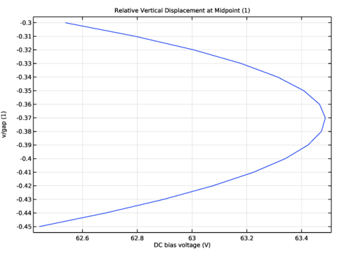
In the Settings window for Point Probe, type Relative Vertical Displacement at Midpoint in the Label text field.
3
In the Variable name text field, type vmid.
4
5
Locate the Expression section. In the Expression text field, type v/gap.
6
Locate the Integration Settings section. From the Method list, choose Summation over nodes.
7
From the Frame list, choose Material.
8
Click the  Show More Options button in the Model Builder toolbar.
9
In the Show More Options dialog, in the tree, select the checkbox for the node Physics > Equation Contributions.
10
Electrostatics (es)
Global Equations 1 (ODE1)
1
In the Physics toolbar, click  Global and choose Global Equations.
2
In the Settings window for Global Equations, locate the Global Equations section.
3
4
Locate the Units section. Click  Select Dependent Variable Quantity.
5
In the Physical Quantity dialog, select Electromagnetics > Electric potential (V) in the tree.
6
This equation will effectively constrain the relative displacement at the midpoint of the beam to a certain value. The DC bias voltage will be a global DOF variable that will play the role of a reaction force associated with this constraint. Thus, the electrostatic load due to the applied Vdc voltage will be computed automatically so that the beam midpoint will be displaced to the desired location.
Add Study
1
In the Home toolbar, click  Add Study to open the Add Study window.
2
Go to the Add Study window.
3
Find the Studies subsection. In the Select Study tree, select General Studies > Stationary.
4
5
In the Home toolbar, click  Add Study to close the Add Study window.
Use the solution of the previous study as initial values of variables solved for.
Study 2
Step 1: Stationary
1
In the Settings window for Stationary, click to expand the Values of Dependent Variables section.
2
Find the Initial values of variables solved for subsection. From the Settings list, choose User controlled.
3
From the Method list, choose Solution.
4
From the Study list, choose Stationary, Stationary.
5
Click to expand the Results While Solving section. From the Probes list, choose None.
Set up a parametric sweep over the displacement of the midpoint, vrel.
6
Click to expand the Study Extensions section. Select the Auxiliary sweep checkbox.
7
8
9
In the Study toolbar, click  Show Default Plots.
The problem is strongly coupled and nonlinear due to the presence of the global equation, so the solver settings need to be adjusted accordingly.
Solver Configurations
In the Model Builder window, expand the Study 2 > Solver Configurations node.
Solution 2 (sol2)
1
In the Model Builder window, expand the Study 2 > Solver Configurations > Solution 2 (sol2) node.
2
Right-click Stationary Solver 1 and choose Fully Coupled.
3
In the Settings window for Fully Coupled, click to expand the Method and Termination section.
4
From the Nonlinear method list, choose Automatic highly nonlinear (Newton).
5
In the Model Builder window, click Study 2.
6
In the Settings window for Study, type Pull In in the Label text field.
7
In the Study toolbar, click  Compute.
Results
Pull-In Plot
1
In the Results toolbar, click  1D Plot Group.
2
In the Settings window for 1D Plot Group, type Pull-In Plot in the Label text field.
3
Locate the Data section. From the Dataset list, choose Pull In/Solution 2 (sol2).
4
Locate the Plot Settings section.
5
Select the y-axis label checkbox. In the associated text field, type v/gap (1).
6
Locate the Legend section. Clear the Show legends checkbox.
Global 1
1
Right-click Pull-In Plot and choose Global.
2
In the Settings window for Global, click Replace Expression in the upper-right corner of the y-Axis Data section. From the menu, choose Component 1 (comp1) > Definitions > vmid - Relative Vertical Displacement at Midpoint - 1.
3
Locate the x-Axis Data section. From the Parameter list, choose Expression.
4
Click Insert Expression (Ctrl+Space) in the upper-right corner of the x-Axis Data section. From the menu, choose Component 1 (comp1) > Electrostatics > Vdc - DC bias voltage - V.
5
Locate the x-Axis Data section. In the Expression text field, type Vdc.
6
In the Pull-In Plot toolbar, click  Plot.
7
Click the  Zoom Extents button in the Graphics toolbar.
Compare the resulting plot with Figure 1.
Determine the pull-in voltage.
Pull-In Voltage
1
In the Results toolbar, click  Global Evaluation.
2
In the Settings window for Global Evaluation, type Pull-In Voltage in the Label text field.
3
Locate the Data section. From the Dataset list, choose Pull In/Solution 2 (sol2).
4
Click Replace Expression in the upper-right corner of the Expressions section. From the menu, choose Component 1 (comp1) > Electrostatics > Vdc - DC bias voltage - V.
5
Locate the Data Series Operation section. From the Transformation list, choose Maximum.
6
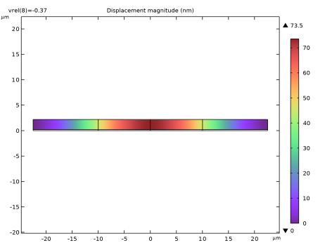
Select the Include vrel checkbox.
7
Click  Evaluate.
The pull-in voltage should be around 63.3 V, for which the beam middle point will be moved downward about 37% of the gap.
Pull-In Displacement
1
In the Model Builder window, under Results click Displacement (solid).
2
In the Settings window for 2D Plot Group, type Pull-In Displacement in the Label text field.
3
Locate the Data section. From the Parameter value (vrel) list, choose -0.37.
4
Locate the Plot Settings section. From the Frame list, choose Material  (X, Y, Z).
5
Locate the Color Legend section. Select the Show maximum and minimum values checkbox.
Surface 1
1
In the Model Builder window, expand the Pull-In Displacement node, then click Surface 1.
2
In the Settings window for Surface, locate the Expression section.
3
From the Unit list, choose nm.
4
In the Pull-In Displacement toolbar, click  Plot.
Compare the resulting plot with Figure 2.