COMSOL 6.4 - Normal Modes of a Biased Resonator

Silicon micromechanical resonators have long been used for designing sensors and are now becoming increasingly important as oscillators in the consumer electronics market. In this sequence of models, a surface micromachined MEMS resonator, designed as part of a micromechanical filter, is analyzed in detail. The resonator is based on that developed in Ref. 1.

This model performs a modal analysis on the resonator, with and without an applied DC bias. The analysis begins from the stationary analysis performed in the accompanying model Stationary Analysis of a Biased Resonator — 2D; please review this model first.

Model Definition

The geometry, fabrication, and operation of the device are discussed for the “Stationary Analysis of a Biased Resonator” model.

This model performs a modal analysis on the structure, with and without applied DC voltage biases of different magnitudes. The bias already exists as a parameter in the model so the prestressed eigenfrequency solver needs no adjustment to the physics settings. To compute the unbiased eigenfrequency, the solver settings are adjusted to solve only the structural mechanics problem.

Results and Discussion

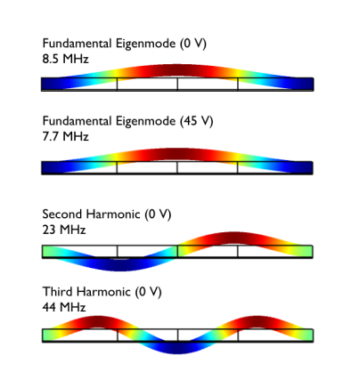
Figure 1 shows the mode shapes for the resonator under different bias conditions.

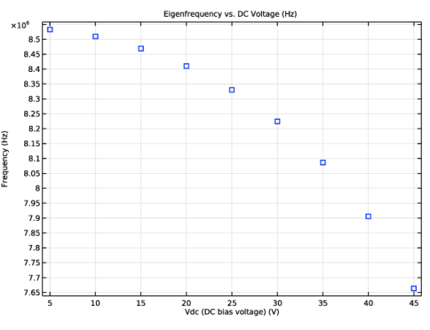
The mode shape does not change significantly with applied bias and the first three modes have the expected shapes for a clamped-clamped beam. The frequency of the fundamental is reduced significantly by the applied bias, an effect known as spring softening (the response of higher-order modes was not computed as a function of applied bias).

Figure 1: Mode shapes for the resonator under different bias conditions. The mode frequencies are indicated in the figure. The colors visualize the relative y-displacement magnitude.

The spring softening effect can be seen in detail in Figure 2. A clear decrease in the resonant frequency is evident with increasing bias voltage. This figure should be compared with Figure 16 of Ref. 1, where the same effect is apparent.

Figure 2: Mode frequency shown against the applied DC voltage bias. The spring softening effect is evident. Compare with Fig. 16 of Ref. 1.

Notes About the COMSOL Implementation

This model excludes certain dependent variables from the solver settings in order to compute the unbiased eigenfrequency. By not computing for the electric potential or the displacement of the air domains, the model is equivalent to a pure solid mechanics problem, solved in the absence of external forces. Excluding dependent variables in the solver in this manner can be useful for debugging models as well as for computing uncoupled problems in this manner.

Reference

1. F.D. Bannon, J.R. Clark, and C. T.-C. Nguyen, “High-Q HF Microelectromechanical Filters,” IEEE J. Solid State Circuits, vol. 35, no. 4, pp. 512–526, 2000.

MEMS_Module/Actuators/biased_resonator_2d_modes

Modeling Instructions

Start from the existing stationary model.

Application Libraries

From the menu, choose .

In the window, select > > in the tree.

Click

Add an unbiased eigenfrequency study. The settings for this study need to be modified so that only the structural part of the problem is solved.

Add Study

In the toolbar, click

to open the window.

Go to the window.

Find the subsection. In the tree, select > .

Click the button in the window toolbar.

In the toolbar, click

to close the window.

Study 2

Step 1: Eigenfrequency

In the window for , locate the section.

Select the checkbox. In the associated text field, type 3.

Click to expand the section. In the table, enter the following settings:


Interface	Output
Electrostatics (es)	None
Moving mesh (Component 1)	None

In the window, click .

In the window for , type Unbiased Eigenfrequency in the text field.

Set up the solver to solve only for the solid mechanics variables.

Solution 2 (sol2)

In the toolbar, click

In the window, click .

Locate the section. Clear the checkbox.

In the toolbar, click

Set the dataset to be in the material frame for postprocessing. This allows the use of the deformation plot attribute.

Results

Unbiased Eigenfrequency/Solution 2 (sol2)

In the window, expand the > node, then click .

In the window for , locate the section.

From the list, choose .

Plot the mode shapes.

Unbiased Modes

In the toolbar, click

In the window for , locate the section.

From the list, choose .

In the text field, type Unbiased Modes.

Surface 1

Right-click and choose .

In the window for , locate the section.

In the text field, type v.

Deformation 1

Right-click and choose .

In the toolbar, click

Click the

button in the toolbar.

Compare the mode shapes with those shown in Figure 1 for all the modes computed. To switch between the modes click and choose a different value from the list.

Root

Add an study.

Add Study

In the toolbar, click