PDF

Dynamics of a Roller Conveyor
Introduction
Roller conveyors are commonly used in warehouses, manufacturing units and baggage handling applications to transport objects from one place to other by gravity, power, or manually. A typical roller conveyor consists of an array of moving rollers arranged either in a straight or curved manner and supported by frames. It is generally made of plastic, mild steel or stainless steel.
This model simulates the dynamics of a roller conveyor transporting a spherical object or a ball. Here, multiple cylindrical rollers are inserted between two C-sectioned beams. Cylindrical guideways are provided on both sides of the conveyor to prevent the ball falling off from rollers. The rollers are rotating about their axes, while the frames and side guideways are fixed. On reaching the other end, the ball is collected in a rectangular tray. All components of the system are assumed rigid. Using rigid body contact with friction, contact is modeled between ball and rollers, ball and side guideways, as well as ball and the surfaces of the tray. The connection between rollers and the frame is simplified using hinge joints. A transient study is performed to analyze the dynamics of ball, contact and friction forces, and energy dissipation due to friction.
Model Definition
The model geometry consists of thirty identical cylindrical rollers of outer radius 24 mm and inner radius 21 mm, and width 450 mm. The rollers are inserted between two curved C-sectioned beams of flange width 100 mm and thickness 5 mm each. The frames’ web height and thickness are 40 mm and 7 mm, respectively.
A spherical ball of radius 180 mm, under the gravity load, is placed on the first roller. As shown in Figure 1, five cylindrical rods are placed as guideways on each side of the conveyor to keep the ball on the rollers by preventing falling off while moving. On reaching the other end, the ball is collected in a three-sided rectangular tray, which is kept at the far end of the conveyor. All components of the system are assumed rigid and use the material data for structural steel.
Figure 1: Model geometry of the roller conveyor.
The connections between rollers and frames are modeled through hinge joints, having only one rotational degree of freedom about their axes. The frames, guideways and tray are assumed to be fixed without any translational or rotational motion. All the rollers are rotating at an angular speed of 765 rpm.
For each rigid roller, a point of contact exists with the spherical ball. Using the rigid body contact with friction functionality, the interaction between each roller and ball is modeled as frictional contacts. The coefficient of friction between the ball and rollers is assumed as 0.1. Similar frictional contacts are used to model the interaction of the ball coming in contact with the cylindrical guideways on both sides. As the rollers rotate, the ball moves forward because of these frictional contacts and finally reaches at the end of the conveyor. Here the ball is collected in a three sided rectangular tray. Rigid body contact with friction functionality is again used to model the contact between the ball and bottom surface and far side of the tray. On the other two sides of the tray, the ball is guarded by the cylindrical guideways.
A time dependent study is performed for 8 s, to analyze the dynamics of the ball and rollers. The contact and frictional forces between ball and rollers and energy dissipation due to friction are also studied.
Results and Discussion
Figure 2 shows the displacement in the ball and rollers.
Figure 2: Displacement of different components of roller conveyor system at t = s.
The rotation of rollers is transferred to the ball through contact between rollers and the ball. Because of frictional contact, the ball moves forward. Figure 3 and Figure 4 show the speed and angular speed of the forward moving ball, as a function of time. It is seen from these figures that as the ball moves forward, speed of the ball increases. When it reaches the tray, the speed again decreases.The components of angular velocity of the ball, as a function of time is plotted in Figure 5.
Figure 3: Speed of the ball, as a function of time.
Figure 4: Angular speed of the ball, as a function of time.
Figure 5: Angular velocity of the ball, as a function of time.
Contact and friction forces between the ball and three sample rollers are shown in Figure 6. These three sample rollers are located at the start, middle and end of the roller conveyor system.
When the ball moves forward, it comes in contact with some of the side guides also. Contact and friction forces between the ball and four sample guideways are shown in Figure 7.
Finally, when the ball falls into the tray, it starts contact with the bottom surface of the tray. While moving in the tray, the ball also comes in contact with the far side of the tray for some time. Figure 8 shows contact and friction forces between the ball and the surfaces of the tray. The ball will not touch the other two sides, as they are guarded by side guideways.
Figure 6: Contact and friction forces between the ball and three sample rollers, as a function of time.
Figure 7: Contact and friction forces between the ball and guideways, as a function of time.
Figure 8: Contact and friction forces between the ball and the tray surfaces, as a function of time.
The frictional energy dissipation rate due to the contact between the ball and the three sample rollers is shown in Figure 9. Similarly, the frictional energy dissipation rate due to the contact between the ball and the side guideways is shown in Figure 10. Figure 11 shows the frictional energy dissipation rate due to the contact between the ball and the surfaces of the tray.
Figure 9: Frictional energy dissipation rate between the ball and three sample rollers, as a function of time.
Figure 10: Frictional energy dissipation rate between the ball and guideways, as a function of time.
Figure 11: Frictional energy dissipation rate between the ball and tray surfaces, as a function of time.
Notes About the COMSOL Implementation
In this model, all components are modeled as rigid elements using Rigid Material nodes, which can be created automatically using the Create Rigid Domains button in the Automated Model Setup section in the Settings window for the Multibody Dynamics interface.
Application Library path: Multibody_Dynamics_Module/Tutorials/roller_conveyor_dynamics
Modeling Instructions
From the File menu, choose New.
New
In the New window, click  Model Wizard.
Model Wizard
1
In the Model Wizard window, click  3D.
2
In the Select Physics tree, select Structural Mechanics > Multibody Dynamics (mbd).
3
Click Add.
4
Click  Study.
5
In the Select Study tree, select General Studies > Time Dependent.
6
Global Definitions
Parameters 1
1
In the Model Builder window, under Global Definitions click Parameters 1.
2
In the Settings window for Parameters, locate the Parameters section.
3
Click  Load from File.
4
If you do not want to import the geometry and create selections, you can load the geometry sequence from the stored model. In the Model Builder window, under Component 1 (comp1) right-click Geometry 1 and choose Insert Sequence. Browse to the model’s Application Libraries folder and double-click the file roller_conveyor_dynamics.mph. You can then continue to the ADD MATERIAL section below.
To import the geometry and create selections from scratch, continue here.
Geometry 1
Import 1 (imp1)
1
In the Model Builder window, expand the Component 1 (comp1) > Geometry 1 node.
2
Right-click Geometry 1 and choose Import.
3
In the Settings window for Import, locate the Source section.
4
Click  Browse.
5
6
Click  Import.
7
Click to expand the Selections of Resulting Entities section. Select the Resulting objects selection checkbox.
8
Select the Individual object selections checkbox.
9
From the Show in physics list, choose All levels.
Ball
1
In the Geometry toolbar, click  Selections and choose Explicit Selection.
2
In the Settings window for Explicit Selection, type Ball in the Label text field.
3
On the object imp1(14), select Domain 1 only.
4
Locate the Color section. From the Color list, choose None or — if you are running the cross-platform desktop —Custom. On the cross-platform desktop, click the Color button.
5
Click Define custom colors.
6
7
Click Add to custom colors.
8
Click Show color palette only or OK on the cross-platform desktop.
9
Click  Build Selected.
Ball Boundaries
1
In the Geometry toolbar, click  Selections and choose Adjacent Selection.
2
In the Settings window for Adjacent Selection, type Ball Boundaries in the Label text field.
3
Locate the Input Entities section. Click  Add.
4
In the Add dialog, select Ball in the Input selections list.
5
Frames
1
In the Geometry toolbar, click  Selections and choose Explicit Selection.
2
In the Settings window for Explicit Selection, type Frames in the Label text field.
3
On the object imp1(1), select Domain 1 only.
4
On the object imp1(23), select Domain 1 only.
5
Locate the Color section. From the Color list, choose None or — if you are running the cross-platform desktop —Custom. On the cross-platform desktop, click the Color button.
6
Click Define custom colors.
7
8
Click Add to custom colors.
9
Click Show color palette only or OK on the cross-platform desktop.
10
Click  Build Selected.
Guides
1
In the Geometry toolbar, click  Selections and choose Explicit Selection.
2
In the Settings window for Explicit Selection, type Guides in the Label text field.
3
On the object imp1(17), select Domain 1 only.
4
On the object imp1(2), select Domains 1 and 2 only.
5
On the object imp1(22), select Domain 1 only.
6
On the object imp1(25), select Domain 1 only.
7
On the object imp1(26), select Domain 1 only.
8
On the object imp1(29), select Domain 1 only.
9
On the object imp1(3), select Domain 1 only.
10
On the object imp1(33), select Domains 1 and 2 only.
11
Locate the Color section. From the Color list, choose None or — if you are running the cross-platform desktop —Custom. On the cross-platform desktop, click the Color button.
12
Click Define custom colors.
13
14
Click Add to custom colors.
15
Click Show color palette only or OK on the cross-platform desktop.
16
Click  Build Selected.
17
In the Home toolbar, click Desktop Layout and choose Reset Desktop.
Tray
1
In the Geometry toolbar, click  Selections and choose Explicit Selection.
2
In the Settings window for Explicit Selection, type Tray in the Label text field.
3
On the object imp1(42), select Domains 1 and 2 only.
4
Locate the Color section. From the Color list, choose None or — if you are running the cross-platform desktop —Custom. On the cross-platform desktop, click the Color button.
5
Click Define custom colors.
6
7
Click Add to custom colors.
8
Click Show color palette only or OK on the cross-platform desktop.
9
Click  Build Selected.
Rollers
1
In the Geometry toolbar, click  Selections and choose Difference Selection.
2
In the Settings window for Difference Selection, type Rollers in the Label text field.
3
Locate the Input Entities section. Click the  Add button for Selections to add.
4
In the Add dialog, select Import 1 in the Selections to add list.
5
6
In the Settings window for Difference Selection, locate the Input Entities section.
7
Click the  Add button for Selections to subtract.
8
In the Add dialog, in the Selections to subtract list, choose Ball, Frames, Guides, and Tray.
9
10
In the Settings window for Difference Selection, locate the Color section.
11
From the Color list, choose None or — if you are running the cross-platform desktop —Custom. On the cross-platform desktop, click the Color button.
12
Click Define custom colors.
13
14
Click Add to custom colors.
15
Click Show color palette only or OK on the cross-platform desktop.
16
Click  Build Selected.
Rollers Boundaries
1
In the Model Builder window, under Component 1 (comp1) > Geometry 1 right-click Ball Boundaries (adjsel1) and choose Duplicate.
2
In the Settings window for Adjacent Selection, type Rollers Boundaries in the Label text field.
3
Locate the Input Entities section. In the Input selections list box, select Ball.
4
Click  Delete.
5
6
In the Add dialog, select Rollers in the Input selections list.
7
8
In the Settings window for Adjacent Selection, locate the Input Entities section.
9
In the Input selections list box, select Rollers.
10
Click  Build Selected.
Fixed Boundaries
1
In the Model Builder window, under Component 1 (comp1) > Geometry 1 right-click Rollers (difsel1) and choose Duplicate.
2
In the Settings window for Difference Selection, type Fixed Boundaries in the Label text field.
3
Locate the Geometric Entity Level section. From the Level list, choose Boundary.
4
Locate the Input Entities section. Click the  Add button for Selections to add.
5
In the Add dialog, select Import 1 in the Selections to add list.
6
7
In the Settings window for Difference Selection, locate the Input Entities section.
8
Click the  Add button for Selections to subtract.
9
In the Add dialog, in the Selections to subtract list, choose Ball Boundaries and Rollers Boundaries.
10
11
In the Settings window for Difference Selection, locate the Color section.
12
From the Color list, choose None.
13
Click  Build Selected.
Ball (sel1), Ball Boundaries (adjsel1), Fixed Boundaries (difsel2), Frames (sel2), Guides (sel3), Rollers (difsel1), Rollers Boundaries (adjsel2), Tray (sel4)
1
In the Model Builder window, under Component 1 (comp1) > Geometry 1, Ctrl-click to select Ball (sel1), Ball Boundaries (adjsel1), Frames (sel2), Guides (sel3), Tray (sel4), Rollers (difsel1), Rollers Boundaries (adjsel2), and Fixed Boundaries (difsel2).
2
Selections
In the Settings window for Group, type Selections in the Label text field.
Form Union (fin)
1
In the Model Builder window, under Component 1 (comp1) > Geometry 1 click Form Union (fin).
2
In the Settings window for Form Union/Assembly, locate the Form Union/Assembly section.
3
From the Action list, choose Form an assembly.
4
Clear the Create pairs checkbox.
5
Click  Build Selected.
Add Material
1
In the Materials toolbar, click  Add Material to open the Add Material window.
2
Go to the Add Material window.
3
In the tree, select Built-in > Structural steel.
4
Click the Add to Component button in the window toolbar.
5
In the Materials toolbar, click  Add Material to close the Add Material window.
Multibody Dynamics (mbd)
Do as follows to generate Rigid Material nodes for all components.
1
In the Settings window for Multibody Dynamics, click Physics Node Generation in the upper-right corner of the Automated Model Setup section. From the menu, choose Create Rigid Domains.
Rigid Material: Left Frame
1
In the Model Builder window, expand the Rigid Domains (All) node, then click Rigid Material 1.
2
In the Settings window for Rigid Material, type Rigid Material: Left Frame in the Label text field.
Rigid Materials
1
Similarly rename other Rigid Material nodes using the information given in the table below.
2
In the Model Builder window, click Rigid Material: Left Frame.
Fixed Constraint 1
In the Physics toolbar, click  Attributes and choose Fixed Constraint.
Similarly add Fixed Constraint nodes to Rigid Material: Right Frame, Rigid Material: Guide L1, Rigid Material: Guide L2, Rigid Material: Guide L3, Rigid Material: Guide L4, Rigid Material: Guide L5, Rigid Material: Guide R1, Rigid Material: Guide R2, Rigid Material: Guide R3, Rigid Material: Guide R4, Rigid Material: Guide R5 and Rigid Material: Tray.
Do as follows to generate Hinge Joint nodes between rollers and left frame.
Hinge Joint 1
1
In the Physics toolbar, click  Global and choose Hinge Joint.
2
In the Settings window for Hinge Joint, locate the Attachment Selection section.
3
From the Source list, choose Rigid Material: Left Frame.
4
From the Destination list, choose Rigid Material: Roller 1.
Center of Joint: Boundary 1
1
In the Model Builder window, click Center of Joint: Boundary 1.
2
In the Settings window for Center of Joint: Boundary, locate the Boundary Selection section.
3
From the Selection list, choose Object 4 (Import 1).
Hinge Joint 1
1
In the Model Builder window, click Hinge Joint 1.
2
In the Settings window for Hinge Joint, locate the Axis of Joint section.
3
From the list, choose Select a parallel edge.
Joint Axis 1
1
In the Model Builder window, click Joint Axis 1.
2
Hinge Joint 1
In the Model Builder window, click Hinge Joint 1.
Prescribed Motion 1
1
In the Physics toolbar, click  Attributes and choose Prescribed Motion.
2
In the Settings window for Prescribed Motion, locate the Prescribed Rotational Motion section.
3
From the Prescribed motion through list, choose Angular velocity.
4
In the ωp text field, type -omega.
Hinge Joints
Similarly create twenty nine more Hinge Joint nodes between left frame and rollers by duplicating Hinge Joint 1 and resetting the inputs using the information given in the table below.
In the Model Builder window, under Component 1 (comp1) > Multibody Dynamics (mbd), Ctrl-click to select Hinge Joint 1 to Hinge Joint 30. Right-click and choose Group.
Hinge Joints
1
In the Model Builder window, under Component 1 (comp1) > Multibody Dynamics (mbd) click Group 2.
2
In the Settings window for Group, type Hinge Joints in the Label text field.
Do as follows to generate Rigid Body Contact nodes between the ball and rollers.
Rigid Body Contact 1
1
In the Physics toolbar, click  Global and choose Rigid Body Contact.
2
In the Settings window for Rigid Body Contact, locate the Source section.
3
From the Source list, choose Rigid Material: Ball.
4
Locate the Destination section. From the Shape list, choose Cylindrical.
5
From the Destination list, choose Rigid Material: Roller 1.
6
Select the Use finite length checkbox.
7
Locate the Contact Settings section. In the fp text field, type fp.
Friction 1
1
In the Physics toolbar, click  Attributes and choose Friction.
2
In the Settings window for Friction, locate the Friction section.
3
In the μ text field, type mu.
4
In the v0 text field, type mbd.diag*1e-3[1/s]*10.
Ball-Rollers Contacts
Similarly create twenty nine more Rigid Body Contact nodes between the ball and rollers by duplicating Rigid Body Contact 1 and resetting the inputs using the information given in the table below.
Add Rigid Body Contact nodes between the ball and side guides by duplicating Rigid Body Contact 30 and resetting the input values.
Rigid Body Contact 31
1
Right-click Friction 1 and choose Duplicate.
2
In the Settings window for Rigid Body Contact, locate the Destination section.
3
From the Destination list, choose Rigid Material: Guide L1.
Ball-Guides Contacts
Similarly create nine more Rigid Body Contact nodes between the ball and side guides by duplicating Rigid Body Contact 31 and resetting the inputs using the information given in the table below.
Add Rigid Body Contact nodes between the ball and tray surfaces by duplicating Rigid Body Contact 40 and resetting the input values.
Rigid Body Contact 41
1
In the Model Builder window, under Component 1 (comp1) > Multibody Dynamics (mbd) right-click Rigid Body Contact 40 and choose Duplicate.
2
In the Settings window for Rigid Body Contact, locate the Destination section.
3
From the Shape list, choose Planar.
4
Locate the Boundary Selection, Destination section. Click to select the  Activate Selection toggle button.
5
Rigid Body Contact 42
1
Right-click Rigid Body Contact 41 and choose Duplicate.
2
In the Settings window for Rigid Body Contact, locate the Boundary Selection, Destination section.
3
Click  Clear Selection.
4
In the Model Builder window, under Component 1 (comp1) > Multibody Dynamics (mbd), Ctrl-click to select Rigid Body Contact 1 to Rigid Body Contact 30. Right-click and choose Group.
Ball-Rollers Contacts
1
In the Model Builder window, under Component 1 (comp1) > Multibody Dynamics (mbd) click Group 3.
2
In the Settings window for Group, type Ball-Rollers Contacts in the Label text field.
Rigid Body Contact 31, Rigid Body Contact 32, Rigid Body Contact 33, Rigid Body Contact 34, Rigid Body Contact 35, Rigid Body Contact 36, Rigid Body Contact 37, Rigid Body Contact 38, Rigid Body Contact 39, Rigid Body Contact 40
1
In the Model Builder window, under Component 1 (comp1) > Multibody Dynamics (mbd), Ctrl-click to select Rigid Body Contact 31, Rigid Body Contact 32, Rigid Body Contact 33, Rigid Body Contact 34, Rigid Body Contact 35, Rigid Body Contact 36, Rigid Body Contact 37, Rigid Body Contact 38, Rigid Body Contact 39, and Rigid Body Contact 40.
2
Ball-Guides Contacts
In the Settings window for Group, type Ball-Guides Contacts in the Label text field.
Rigid Body Contact 41, Rigid Body Contact 42
1
In the Model Builder window, under Component 1 (comp1) > Multibody Dynamics (mbd), Ctrl-click to select Rigid Body Contact 41 and Rigid Body Contact 42.
2
Ball-Tray Contacts
In the Settings window for Group, type Ball-Tray Contacts in the Label text field.
Gravity 1
In the Physics toolbar, click  Global and choose Gravity.
Mesh 1
Free Triangular 1
1
In the Mesh toolbar, click  More Generators and choose Free Triangular.
2
In the Settings window for Free Triangular, locate the Boundary Selection section.
3
Click  Paste Selection.
4
In the Paste Selection dialog, type 13, 19, 23, 29, 39, 49, 59, 69, 79, 89, 99, 109, 119, 137, 147, 157, 162, 163, 173, 183, 193, 203, 219, 229, 234, 235, 240, 241, 251, 261, 266, 267, 277, 290, 297, 302, 312, 322, 332, 342, 352, 362, 372, 382 in the Selection text field.
5
Size 1
1
Right-click Free Triangular 1 and choose Size.
2
In the Settings window for Size, locate the Element Size section.
3
From the Predefined list, choose Finer.
Size
1
In the Model Builder window, under Component 1 (comp1) > Mesh 1 click Size.
2
In the Settings window for Size, locate the Element Size section.
3
From the Predefined list, choose Finer.
Mapped 1
1
In the Mesh toolbar, click  More Generators and choose Mapped.
2
Distribution 1
1
Right-click Mapped 1 and choose Distribution.
2
3
In the Settings window for Distribution, locate the Distribution section.
4
In the Number of elements text field, type 25.
Swept 1
1
In the Mesh toolbar, click  Swept.
2
In the Settings window for Swept, locate the Domain Selection section.
3
From the Geometric entity level list, choose Domain.
4
From the Selection list, choose All domains.
5
Distribution 1
1
Right-click Swept 1 and choose Distribution.
2
In the Settings window for Distribution, locate the Domain Selection section.
3
From the Selection list, choose Frames.
4
Locate the Distribution section. In the Number of elements text field, type 50.
Distribution 2
1
In the Model Builder window, right-click Swept 1 and choose Distribution.
2
In the Settings window for Distribution, locate the Domain Selection section.
3
From the Selection list, choose Guides.
4
Locate the Distribution section. In the Number of elements text field, type 20.
Distribution 3
1
Right-click Swept 1 and choose Distribution.
2
In the Settings window for Distribution, locate the Domain Selection section.
3
From the Selection list, choose Rollers.
4
Locate the Distribution section. In the Number of elements text field, type 10.
Free Tetrahedral 1
In the Mesh toolbar, click  Free Tetrahedral.
Size 1
1
Right-click Free Tetrahedral 1 and choose Size.
2
In the Settings window for Size, locate the Element Size section.
3
From the Predefined list, choose Finer.
4
Locate the Geometric Entity Selection section. From the Geometric entity level list, choose Domain.
5
Size 2
1
In the Model Builder window, right-click Free Tetrahedral 1 and choose Size.
2
In the Settings window for Size, locate the Geometric Entity Selection section.
3
From the Geometric entity level list, choose Domain.
4
5
Locate the Element Size section. Click the Custom button.
6
Locate the Element Size Parameters section.
7
Select the Maximum element size checkbox. In the associated text field, type 0.03.
8
Click  Build All.
Study 1
Step 1: Time Dependent
1
In the Model Builder window, under Study 1 click Step 1: Time Dependent.
2
In the Settings window for Time Dependent, locate the Study Settings section.
3
In the Output times text field, type range(0,0.01,8).
4
Click to expand the Results While Solving section. Select the Plot checkbox.
Solution 1 (sol1)
1
In the Study toolbar, click  Show Default Solver.
2
In the Model Builder window, expand the Solution 1 (sol1) node.
3
In the Model Builder window, expand the Study 1 > Solver Configurations > Solution 1 (sol1) > Time-Dependent Solver 1 node, then click Fully Coupled 1.
4
In the Settings window for Fully Coupled, click to expand the Method and Termination section.
5
In the Maximum number of iterations text field, type 15.
6
In the Model Builder window, under Study 1 > Solver Configurations > Solution 1 (sol1) click Time-Dependent Solver 1.
7
In the Settings window for Time-Dependent Solver, click to expand the Time Stepping section.
8
From the Steps taken by solver list, choose Intermediate.
9
In the Study toolbar, click  Compute.
Results
Click the  Show Grid button in the Graphics toolbar.
Follow the instructions below to plot system displacement as shown in Figure 2.
Displacement (mbd)
In the Model Builder window, expand the Results > Displacement (mbd) node.
Selection 1
1
In the Model Builder window, expand the Results > Displacement (mbd) > Surface node.
2
Right-click Surface and choose Selection.
3
In the Settings window for Selection, locate the Selection section.
4
From the Selection list, choose Ball Boundaries.
Surface 2
In the Model Builder window, right-click Surface and choose Duplicate.
Selection 1
1
In the Model Builder window, expand the Surface 2 node, then click Selection 1.
2
In the Settings window for Selection, locate the Selection section.
3
From the Selection list, choose Rollers Boundaries.
Surface 2
1
In the Model Builder window, click Surface 2.
2
In the Settings window for Surface, click to expand the Title section.
3
From the Title type list, choose None.
4
Locate the Coloring and Style section. Clear the Color legend checkbox.
5
From the Color table list, choose WaveLight.
Surface 3
Right-click Results > Displacement (mbd) > Surface 2 and choose Duplicate.
Selection 1
1
In the Model Builder window, expand the Surface 3 node, then click Selection 1.
2
In the Settings window for Selection, locate the Selection section.
3
From the Selection list, choose Fixed Boundaries.
Surface 3
1
In the Model Builder window, click Surface 3.
2
In the Settings window for Surface, locate the Coloring and Style section.
3
From the Coloring list, choose Uniform.
4
From the Color list, choose Gray.
Transparency 1
1
Right-click Surface 3 and choose Transparency.
2
Click the  Zoom Extents button in the Graphics toolbar.
3
In the Displacement (mbd) toolbar, click  Plot.
Follow the instructions below to plot speed of the ball. The resulting plot should match the one shown in Figure 3.
Speed [Ball]
1
In the Results toolbar, click  1D Plot Group.
2
In the Settings window for 1D Plot Group, type Speed [Ball] in the Label text field.
3
Click to expand the Title section. From the Title type list, choose Label.
4
Locate the Legend section. Clear the Show legends checkbox.
Global 1
1
Right-click Speed [Ball] and choose Global.
2
In the Settings window for Global, locate the y-Axis Data section.
3
Speed [Ball]
1
In the Model Builder window, click Speed [Ball].
2
In the Settings window for 1D Plot Group, locate the Plot Settings section.
3
Select the x-axis label checkbox.
4
Select the y-axis label checkbox.
5
In the Speed [Ball] toolbar, click  Plot.
Follow the instructions below to plot angular speed of the ball. The resulting plot should match the one shown in Figure 4.
Angular Speed [Ball]
1
Right-click Speed [Ball] and choose Duplicate.
2
In the Settings window for 1D Plot Group, type Angular Speed [Ball] in the Label text field.
3
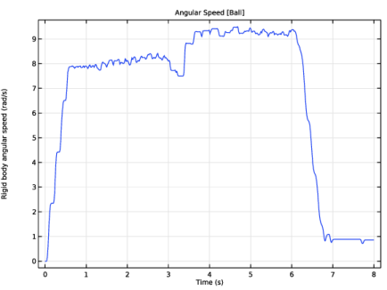
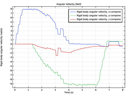
Locate the Plot Settings section. In the y-axis label text field, type Rigid body angular speed (rad/s).
Global 1
1
In the Model Builder window, expand the Angular Speed [Ball] node, then click Global 1.
2
In the Settings window for Global, locate the y-Axis Data section.
3
Angular Speed [Ball]
1
In the Model Builder window, click Angular Speed [Ball].
2
In the Angular Speed [Ball] toolbar, click  Plot.
Follow the instructions below to plot angular velocity of the ball. The resulting plot should match the one shown in Figure 5.
Angular Velocity [Ball]
1
Right-click Angular Speed [Ball] and choose Duplicate.
2
In the Settings window for 1D Plot Group, type Angular Velocity [Ball] in the Label text field.
3
Locate the Plot Settings section. In the y-axis label text field, type Rigid body angular velocity (rad/s).
4
Locate the Legend section. Select the Show legends checkbox.
Global 1
1
In the Model Builder window, expand the Angular Velocity [Ball] node, then click Global 1.
2
In the Settings window for Global, locate the y-Axis Data section.
3
4
In the Angular Velocity [Ball] toolbar, click  Plot.
Follow the instructions below to plot contact and friction force between the ball and three sample rollers. The resulting plot should match the one shown in Figure 6.
Contact & Friction Force [Rollers]
1
In the Model Builder window, right-click Angular Velocity [Ball] and choose Duplicate.
2
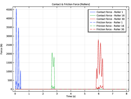
In the Settings window for 1D Plot Group, type Contact & Friction Force [Rollers] in the Label text field.
Global 1
1
In the Model Builder window, expand the Contact & Friction Force [Rollers] node, then click Global 1.
2
In the Settings window for Global, locate the y-Axis Data section.
3
Click  Clear Table.
4
5
Click to expand the Legends section. From the Legends list, choose Manual.
6
Global 2
1
Right-click Results > Contact & Friction Force [Rollers] > Global 1 and choose Duplicate.
2
In the Settings window for Global, locate the y-Axis Data section.
3
4
Click to expand the Coloring and Style section. Find the Line style subsection. From the Line list, choose Dashed.
5
From the Color list, choose Cycle (reset).
6
Locate the Legends section. In the table, enter the following settings:
Contact & Friction Force [Rollers]
1
In the Model Builder window, click Contact & Friction Force [Rollers].
2
In the Settings window for 1D Plot Group, locate the Plot Settings section.
3
In the y-axis label text field, type Force (N).
4
In the Contact & Friction Force [Rollers] toolbar, click  Plot.
Follow the instructions below to plot contact and friction force between the ball and four side guides. The resulting plot should match the one shown in Figure 7.
Contact & Friction Force [Guides]
1
Right-click Contact & Friction Force [Rollers] and choose Duplicate.
2
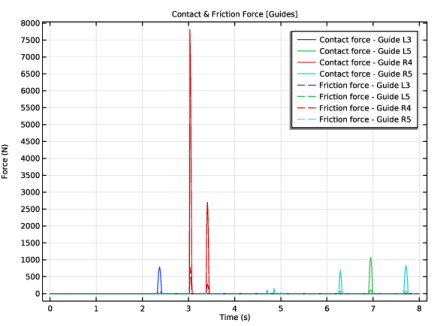
In the Settings window for 1D Plot Group, type Contact & Friction Force [Guides] in the Label text field.
Global 1
1
In the Model Builder window, expand the Contact & Friction Force [Guides] node, then click Global 1.
2
In the Settings window for Global, locate the y-Axis Data section.
3
Click  Clear Table.
4
5
Locate the Legends section. In the table, enter the following settings:
Global 2
1
In the Model Builder window, click Global 2.
2
In the Settings window for Global, locate the y-Axis Data section.
3
4
Locate the Legends section. In the table, enter the following settings:
Contact & Friction Force [Guides]
1
In the Model Builder window, click Contact & Friction Force [Guides].
2
In the Contact & Friction Force [Guides] toolbar, click  Plot.
Follow the instructions below to plot contact and friction force between the ball and tray surfaces. The resulting plot should match the one shown in Figure 8.
Contact & Friction Force [Tray]
1
Right-click Contact & Friction Force [Guides] and choose Duplicate.
2
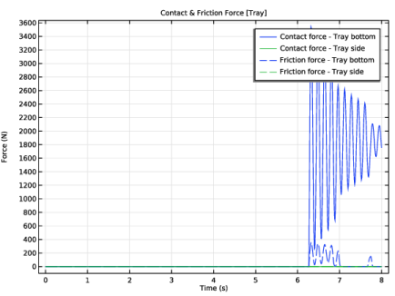
In the Settings window for 1D Plot Group, type Contact & Friction Force [Tray] in the Label text field.
Global 1
1
In the Model Builder window, expand the Contact & Friction Force [Tray] node, then click Global 1.
2
In the Settings window for Global, locate the y-Axis Data section.
3
Click  Clear Table.
4
5
Locate the Legends section. Right-click and choose Select All.
6
7
Global 2
1
In the Model Builder window, click Global 2.
2
In the Settings window for Global, locate the y-Axis Data section.
3
Click  Clear Table.
4
5
Locate the Legends section. Right-click and choose Select All.
6
7
Contact & Friction Force [Tray]
1
In the Model Builder window, click Contact & Friction Force [Tray].
2
In the Contact & Friction Force [Tray] toolbar, click  Plot.
Follow the instructions below to plot frictional energy dissipation rate between the ball and three sample rollers. The resulting plot should match the one shown in Figure 9.
Frictional Energy Dissipation Rate [Rollers]
1
Right-click Contact & Friction Force [Tray] and choose Duplicate.
2
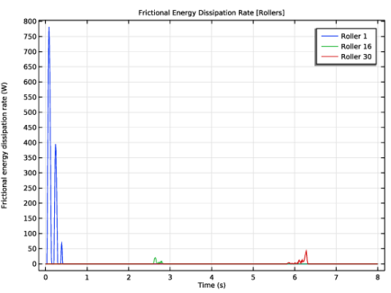
In the Settings window for 1D Plot Group, type Frictional Energy Dissipation Rate [Rollers] in the Label text field.
Global 1
1
In the Model Builder window, expand the Frictional Energy Dissipation Rate [Rollers] node, then click Global 1.
2
In the Settings window for Global, locate the y-Axis Data section.
3
Click  Clear Table.
4
5
Locate the Legends section. In the table, enter the following settings:
Global 2
In the Model Builder window, right-click Global 2 and choose Delete.
Frictional Energy Dissipation Rate [Rollers]
1
In the Model Builder window, under Results click Frictional Energy Dissipation Rate [Rollers].
2
In the Settings window for 1D Plot Group, locate the Plot Settings section.
3
Clear the y-axis label checkbox.
4
In the Frictional Energy Dissipation Rate [Rollers] toolbar, click  Plot.
Follow the instructions below to plot frictional energy dissipation rate between the ball and four sample side guides. The resulting plot should match the one shown in Figure 10.
Frictional Energy Dissipation Rate [Guides]
1
Right-click Frictional Energy Dissipation Rate [Rollers] and choose Duplicate.
2
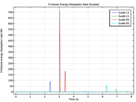
In the Settings window for 1D Plot Group, type Frictional Energy Dissipation Rate [Guides] in the Label text field.
Global 1
1
In the Model Builder window, expand the Frictional Energy Dissipation Rate [Guides] node, then click Global 1.
2
In the Settings window for Global, locate the y-Axis Data section.
3
Click  Clear Table.
4
5
Locate the Legends section. In the table, enter the following settings:
Frictional Energy Dissipation Rate [Guides]
1
In the Model Builder window, click Frictional Energy Dissipation Rate [Guides].
2
In the Frictional Energy Dissipation Rate [Guides] toolbar, click  Plot.
Follow the instructions below to plot frictional energy dissipation rate between the ball and surfaces of tray. The resulting plot should match the one shown in Figure 11.
Frictional Energy Dissipation Rate [Tray]
1
Right-click Frictional Energy Dissipation Rate [Guides] and choose Duplicate.
2
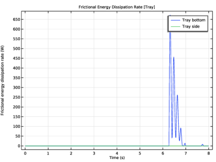
In the Settings window for 1D Plot Group, type Frictional Energy Dissipation Rate [Tray] in the Label text field.
Global 1
1
In the Model Builder window, expand the Frictional Energy Dissipation Rate [Tray] node, then click Global 1.
2
In the Settings window for Global, locate the y-Axis Data section.
3
Click  Clear Table.
4
5
Locate the Legends section. In the table, enter the following settings:
Frictional Energy Dissipation Rate [Tray]
1
In the Model Builder window, click Frictional Energy Dissipation Rate [Tray].
2
In the Frictional Energy Dissipation Rate [Tray] toolbar, click  Plot.
Angular Speed [Ball], Angular Velocity [Ball], Speed [Ball]
1
In the Model Builder window, under Results, Ctrl-click to select Speed [Ball], Angular Speed [Ball], and Angular Velocity [Ball].
2
Speed [Ball]
In the Settings window for Group, type Speed [Ball] in the Label text field.
Contact & Friction Force [Guides], Contact & Friction Force [Rollers], Contact & Friction Force [Tray]
1
In the Model Builder window, under Results, Ctrl-click to select Contact & Friction Force [Rollers], Contact & Friction Force [Guides], and Contact & Friction Force [Tray].
2
Contact & Friction Forces
In the Settings window for Group, type Contact & Friction Forces in the Label text field.
Frictional Energy Dissipation Rate [Guides], Frictional Energy Dissipation Rate [Rollers], Frictional Energy Dissipation Rate [Tray]
1
In the Model Builder window, under Results, Ctrl-click to select Frictional Energy Dissipation Rate [Rollers], Frictional Energy Dissipation Rate [Guides], and Frictional Energy Dissipation Rate [Tray].
2
Frictional Energy Dissipation Rates
In the Settings window for Group, type Frictional Energy Dissipation Rates in the Label text field.
Finally, to generate an animation of the roller conveyor system, follow these instructions:
Displacement (mbd)
1
In the Results toolbar, click  Animation and choose Player.
2
In the Settings window for Animation, type Displacement (mbd) in the Label text field.
3
Locate the Frames section. In the Number of frames text field, type 100.