|
|
|
|
•
|
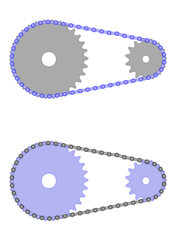
Links: This is a domain selection containing all chain link domains. The selection is used for creating a Rigid Material node for each of the link plates.
|
|
•
|
Sprockets: This is a domain selection containing both sprocket domains. The selection is used for creating a Rigid Material node for each of the sprockets.
|
|
•
|
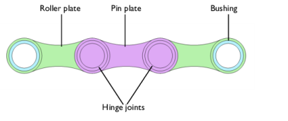
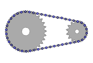
Pin Inner Boundaries: This is a boundary selection containing the inner boundaries of all pin plates. The selection is used for creating an Attachment node for each of the pin plates.
|
|
•
|
Roller Inner Boundaries: This is a boundary selection containing the inner boundaries of the roller plates. The selection is used for creating an Attachment node for each of the roller plates, and it is located at same geometrical position as the Pin Inner Boundaries (Figure 4). Attachments created for the pin and roller plates are used as Source and Destination in Hinge Joint nodes.
|
|
•
|
|
•
|
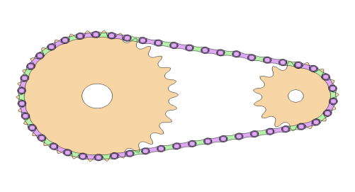
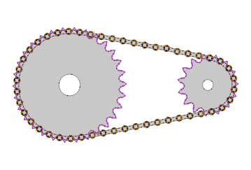
Sprocket Outer Boundaries: This boundary selection contains the outer surfaces of the sprockets. As shown in Figure 5, these are the boundaries which come in contact with chain rollers.
|
|
•
|
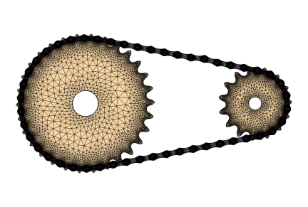
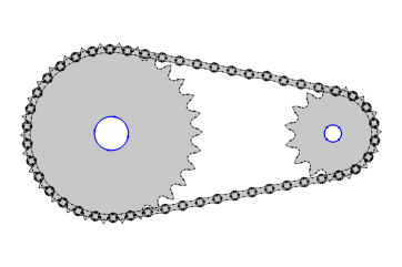
Sprocket Inner Boundaries: This boundary selection contains the inner surfaces of the sprockets, as shown in Figure 6. It is used for creating attachments and hinge joints for mounting the sprockets onto shafts.
|
|
•
|
To build a chain drive system geometry, you can import a roller chain sprocket assembly part from the Part Library, and customize it by changing its input parameters.
|
|
•
|
Chain Drive node operates on the geometry in the assembly state.
|
|
•
|
Chain Drive node creates new physics nodes from selections available in geometry. If you are using part imported from the Part Library, select the checkbox in Geometry to keep noncontributing selections. If you are building a geometry of a roller chain and sprocket assembly, you also need to create appropriate selections for the Chain Drive node to operate.
|
|
•
|
When one or more selection inputs of Chain Drive node change, the selections of the physics nodes created by the Chain Drive node also change. Hence these nodes have to be deleted and recreated. This is indicated by a warning node appearing under the Chain Drive node. In that case, you need to press the Create Links and Joints button. This will automatically create new groups of physics nodes in accordance with the changed selection inputs.
|
|
1
|
|
2
|
|
3
|
Click Add.
|
|
4
|
Click
|
|
5
|
|
6
|
Click
|
|
1
|
|
2
|
|
1
|
|
2
|
|
3
|
|
4
|
|
1
|
|
2
|
|
3
|
|
1
|
|
2
|
In the Part Libraries window, select Multibody Dynamics Module > 2D > Roller Chains > roller_chain_sprocket_assembly_2d in the tree.
|
|
3
|
Click
|
|
4
|
In the Select Part Variant dialog, select Specify sprocket center distance in the Select part variant list.
|
|
5
|
Click OK.
|
|
1
|
In the Model Builder window, under Component 1 (comp1) > Geometry 1 click Roller Chain Sprocket (2D) 1 (pi1).
|
|
2
|
|
3
|
Select the Keep noncontributing selections checkbox.
|
|
4
|
Click
|
|
1
|
|
2
|
|
3
|
|
4
|
Clear the Create pairs checkbox.
|
|
5
|
Click
|
|
1
|
|
2
|
Go to the Add Material window.
|
|
3
|
|
4
|
Click the Add to Component button in the window toolbar.
|
|
5
|
|
1
|
|
2
|
|
1
|
|
2
|
|
3
|
|
4
|
|
5
|
|
1
|
|
2
|
|
3
|
|
4
|
|
1
|
|
2
|
In the Settings window for Chain Drive, click the Create Links and Joints button in the window toolbar.
|
|
1
|
|
2
|
In the Settings window for Mass and Moment of Inertia, locate the Mass and Moment of Inertia section.
|
|
3
|
|
1
|
|
2
|
|
3
|
|
4
|
|
1
|
|
2
|
|
3
|
From the list, choose Joint.
|
|
4
|
|
1
|
In the Model Builder window, under Component 1 (comp1) right-click Definitions and choose Variables.
|
|
2
|
|
1
|
|
2
|
|
3
|
|
4
|
|
5
|
|
6
|
|
7
|
Click
|
|
1
|
|
2
|
|
3
|
|
4
|
|
5
|
In the Model Builder window, expand the Study 1 > Solver Configurations > Solution 1 (sol1) > Time-Dependent Solver 1 node, then click Fully Coupled 1.
|
|
6
|
|
7
|
|
8
|
|
1
|
|
2
|
|
3
|
|
1
|
|
2
|
|
3
|
|
4
|
|
5
|
|
6
|
|
1
|
|
2
|
|
3
|
Click to expand the Title section. Locate the Coloring and Style section. From the Color list, choose Yellow.
|
|
1
|
|
2
|
|
3
|
|
4
|
|
1
|
|
2
|
|
3
|
|
1
|
|
2
|
|
3
|
Click
|
|
1
|
|
2
|
|
3
|
|
4
|
|
5
|
|
1
|
|
2
|
|
3
|
|
1
|
|
2
|
|
3
|
|
4
|
|
1
|
|
2
|
|
3
|
|
4
|
|
1
|
|
2
|
|
3
|
|
4
|
|
1
|
|
2
|
|
3
|
|
4
|
|
1
|
|
2
|
|
3
|
|
1
|
|
2
|
|
3
|
|
1
|
|
2
|
|
3
|
|
4
|
|
5
|
|
1
|
|
2
|
|
3
|
|
4
|
|
1
|
|
2
|
|
3
|
|
4
|
|
1
|
|
2
|
|
3
|
|
4
|
|
5
|
Select the y-axis label checkbox.
|
|
6
|
|
7
|
|
8
|
|
1
|
|
2
|
|
4
|
|
1
|
|
2
|
|
3
|
|
4
|
|
1
|
|
2
|
|
1
|
|
2
|
|
3
|
|
4
|
|
5
|
Select the y-axis label checkbox.
|
|
6
|
|
7
|
|
8
|
|
1
|
|
2
|
|
3
|
|
4
|
|
5
|
Locate the y-Axis Data section. In the table, enter the following settings:
|
|
6
|
|
1
|
|
2
|
|
3
|
|
4
|
Locate the y-Axis Data section. In the table, enter the following settings:
|
|
5
|
Locate the Legends section. In the table, enter the following settings:
|
|
1
|
|
2
|
|
3
|
|
4
|
|
1
|
|
2
|
|
1
|
|
2
|
|
1
|
|
2
|
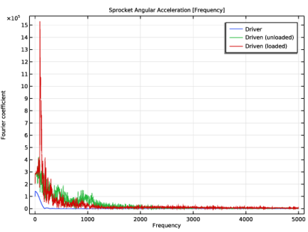
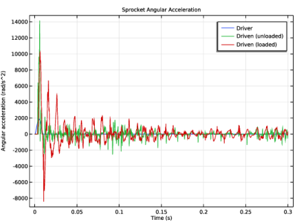
In the Settings window for 1D Plot Group, type Sprocket Angular Acceleration in the Label text field.
|
|
3
|
Locate the Plot Settings section. In the y-axis label text field, type Angular acceleration (rad/s^2).
|
|
1
|
|
2
|
|
1
|
|
2
|
|
3
|
|
4
|
Click
|
|
5
|
|
6
|
|
7
|
Click Add.
|
|
8
|
|
1
|
|
2
|
In the Settings window for 1D Plot Group, type Sprocket Angular Acceleration [Frequency] in the Label text field.
|
|
3
|
|
4
|
Clear the y-axis label checkbox.
|
|
1
|
In the Model Builder window, expand the Sprocket Angular Acceleration [Frequency] node, then click Global 1.
|
|
2
|
|
3
|
|
4
|
|
1
|
|
2
|
|
3
|
|
4
|
|
5
|
|
1
|
|
2
|
|
3
|
|
1
|
|
2
|
|
3
|
|
1
|
|
2
|
|
3
|
|
1
|
|
2
|
|
3
|
|
4
|
|
1
|
|
2
|
|
3
|