
|
|
|
|
•
|
A Joint node can establish a direct connection between Rigid Material nodes. However, for flexible elements, Attachment nodes are needed to define the connection boundaries.
|
|
•
|
Constraint boundary conditions like Prescribed Displacement cannot be used with a Rigid Material node. Hence, the Prescribed Displacement/Rotation node (subnode to Rigid Material) is used to constrain or prescribe the corresponding degrees of freedom.
|
|
•
|
The connections used in the model can be reviewed in the Joints Summary section at the interface settings.
|
|
•
|
The shape function order for flexible components, is by default set to Linear. For better accuracy, you can switch it to Quadratic.
|
|
1
|
|
2
|
|
3
|
Click Add.
|
|
4
|
|
5
|
Click Add.
|
|
6
|
Click
|
|
7
|
|
8
|
Click
|
|
1
|
|
2
|
|
1
|
|
2
|
|
3
|
Click
|
|
4
|
Browse to the model’s Application Libraries folder and double-click the file reciprocating_engine_2d.mphbin.
|
|
5
|
Click
|
|
6
|
|
1
|
|
2
|
|
3
|
|
4
|
|
5
|
|
1
|
|
3
|
|
4
|
Clear the Compute integral in revolved geometry checkbox.
|
|
1
|
|
2
|
|
3
|
|
5
|
|
1
|
|
2
|
|
1
|
|
2
|
Go to the Add Material window.
|
|
3
|
|
4
|
Click the Add to Component button in the window toolbar.
|
|
5
|
|
1
|
|
3
|
|
4
|
Click
|
|
5
|
|
6
|
|
7
|
Click OK.
|
|
8
|
|
9
|
Click
|
|
10
|
|
11
|
|
12
|
Click OK.
|
|
13
|
|
14
|
|
15
|
In the Dependent variables (Pa) table, enter the following settings:
|
|
1
|
In the Model Builder window, under Thermodynamic Analysis (comp1) > Coefficient Form PDE (c) click Coefficient Form PDE 1.
|
|
2
|
|
3
|
|
4
|
|
5
|
|
6
|
|
1
|
|
2
|
|
3
|
|
1
|
In the Model Builder window, under Thermodynamic Analysis (comp1) click Heat Transfer in Fluids (ht).
|
|
1
|
In the Model Builder window, under Thermodynamic Analysis (comp1) > Heat Transfer in Fluids (ht) click Fluid 1.
|
|
2
|
|
3
|
|
1
|
|
3
|
|
4
|
|
1
|
|
2
|
|
3
|
|
4
|
Click
|
|
1
|
|
2
|
|
1
|
|
2
|
|
3
|
|
4
|
|
5
|
|
6
|
Clear the Generate default plots checkbox.
|
|
7
|
|
1
|
|
2
|
|
1
|
|
3
|
|
4
|
|
5
|
|
6
|
|
7
|
|
8
|
|
9
|
|
10
|
|
1
|
|
2
|
|
3
|
|
4
|
|
5
|
|
1
|
|
2
|
|
3
|
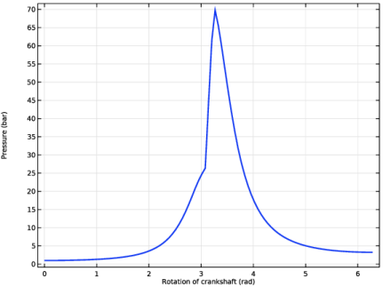
Locate the Plot Settings section. In the x-axis label text field, type Rotation of crankshaft (rad).
|
|
1
|
|
2
|
|
3
|
|
4
|
|
1
|
|
2
|
|
3
|
Click
|
|
4
|
Browse to a suitable folder, enter the filename reciprocating_engine_pressure.txt, and then click Save.
|
|
5
|
|
6
|
Clear the Full precision checkbox.
|
|
7
|
Click the Export button to save the file.
|
|
1
|
|
2
|
|
3
|
|
4
|
Locate the Expressions section. In the table, enter the following settings:
|
|
5
|
Click
|
|
1
|
Go to the Table 1 window.
|
|
1
|
|
2
|
Go to the Add Physics window.
|
|
3
|
|
4
|
Find the Physics interfaces in study subsection. In the table, clear the Solve checkbox for Study: Thermodynamic Analysis.
|
|
5
|
Click the Add to Component 2 button in the window toolbar.
|
|
6
|
|
1
|
|
2
|
Go to the Add Study window.
|
|
3
|
|
4
|
Find the Physics interfaces in study subsection. In the table, clear the Solve checkboxes for Heat Transfer in Fluids (ht) and Coefficient Form PDE (c).
|
|
5
|
Click the Add Study button in the window toolbar.
|
|
6
|
|
1
|
|
2
|
|
3
|
Click
|
|
4
|
Browse to the model’s Application Libraries folder and double-click the file reciprocating_engine.mphbin.
|
|
5
|
Click
|
|
1
|
|
2
|
|
3
|
|
4
|
Clear the Keep interior boundaries checkbox.
|
|
1
|
|
2
|
|
3
|
|
4
|
Click
|
|
5
|
|
6
|
|
7
|
Clear the Automatic detection of small details checkbox.
|
|
1
|
In the Model Builder window, under Multibody Analysis (comp2) > Definitions, Ctrl-click to select Identity Boundary Pair 1 (ap1), Identity Boundary Pair 2 (ap2), Identity Boundary Pair 3 (ap3), Identity Boundary Pair 4 (ap4), Identity Boundary Pair 6 (ap6), and Identity Boundary Pair 8 (ap8).
|
|
2
|
Right-click and choose Group.
|
|
1
|
In the Model Builder window, under Multibody Analysis (comp2) > Definitions, Ctrl-click to select Identity Boundary Pair 5 (ap5), Identity Boundary Pair 7 (ap7), and Identity Boundary Pair 9 (ap9).
|
|
2
|
Right-click and choose Group.
|
|
1
|
|
2
|
|
1
|
|
2
|
|
3
|
Click
|
|
4
|
Browse to the model’s Application Libraries folder and double-click the file reciprocating_engine_pressure.txt.
|
|
5
|
|
6
|
|
7
|
In the Function table, enter the following settings:
|
|
1
|
|
2
|
|
3
|
|
4
|
|
5
|
|
6
|
|
1
|
|
2
|
|
3
|
|
4
|
|
1
|
|
2
|
|
3
|
|
4
|
|
1
|
|
2
|
Click in the Graphics window and then press Ctrl+A to select all domains.
|
|
4
|
|
1
|
|
2
|
Go to the Add Material window.
|
|
3
|
|
4
|
Click the Add to Component button in the window toolbar.
|
|
5
|
|
1
|
|
2
|
|
3
|
Click Physics Node Generation in the upper-right corner of the Automated Model Setup section. From the menu, choose Create Rigid Domains.
|
|
1
|
|
2
|
|
1
|
The details of Hinge Joint nodes between different components of engine are given in the table below:
|
|
2
|
|
3
|
|
4
|
|
5
|
|
6
|
Click Physics Node Generation in the upper-right corner of the Automated Model Setup section. From the menu, choose Create Joints.
|
|
1
|
|
2
|
|
3
|
|
1
|
In the Model Builder window, under Multibody Analysis (comp2) > Multibody Dynamics (mbd) > Hinge Joints click Attachment 2.
|
|
2
|
|
3
|
|
1
|
In the Model Builder window, under Multibody Analysis (comp2) > Multibody Dynamics (mbd) > Hinge Joints right-click Hinge Joint 6 and choose Duplicate.
|
|
2
|
|
3
|
|
4
|
|
5
|
|
6
|
|
1
|
|
1
|
|
1
|
|
2
|
|
3
|
|
4
|
Click Physics Node Generation in the upper-right corner of the Automated Model Setup section. From the menu, choose Create Joints.
|
|
1
|
|
2
|
|
3
|
|
4
|
|
5
|
|
1
|
|
2
|
|
3
|
|
4
|
|
5
|
|
6
|
|
1
|
|
2
|
|
3
|
|
4
|
|
1
|
|
1
|
|
2
|
|
1
|
|
2
|
|
3
|
Specify the M vector as
|
|
1
|
|
2
|
|
3
|
Specify the M vector as
|
|
1
|
|
2
|
|
3
|
|
4
|
|
5
|
|
1
|
|
2
|
|
3
|
|
4
|
|
5
|
|
1
|
|
2
|
|
3
|
|
4
|
|
5
|
|
1
|
In the Model Builder window, under Multibody Analysis (comp2) > Multibody Dynamics (mbd), Ctrl-click to select Boundary Load 1, Boundary Load 2, and Boundary Load 3.
|
|
2
|
Right-click and choose Group.
|
|
1
|
|
2
|
|
3
|
|
4
|
Click
|
|
1
|
|
2
|
|
3
|
|
1
|
|
2
|
|
3
|
In the Model Builder window, expand the Study: Multibody Analysis > Solver Configurations > Solution 2 (sol2) > Dependent Variables 1 node, then click comp2.mbd.att1.Fc1x.
|
|
4
|
|
5
|
|
6
|
In the Model Builder window, under Study: Multibody Analysis > Solver Configurations > Solution 2 (sol2) > Dependent Variables 1 click comp2.mbd.att1.Fd1x.
|
|
7
|
|
8
|
|
9
|
In the Model Builder window, under Study: Multibody Analysis > Solver Configurations > Solution 2 (sol2) > Dependent Variables 1 click comp2.mbd.att2.Fc1x.
|
|
10
|
|
11
|
|
12
|
In the Model Builder window, under Study: Multibody Analysis > Solver Configurations > Solution 2 (sol2) > Dependent Variables 1 click comp2.mbd.att2.Fd1x.
|
|
13
|
|
14
|
|
15
|
In the Model Builder window, under Study: Multibody Analysis > Solver Configurations > Solution 2 (sol2) click Time-Dependent Solver 1.
|
|
16
|
|
17
|
|
18
|
|
19
|
|
20
|
|
1
|
|
2
|
Right-click Results > Datasets > Study: Multibody Analysis/Solution 2 (3) (sol2) and choose Duplicate.
|
|
1
|
|
2
|
|
3
|
|
1
|
|
2
|
|
3
|
|
4
|
|
5
|
|
1
|
|
2
|
|
3
|
|
4
|
|
5
|
|
1
|
|
3
|
|
1
|
|
2
|
Go to the Result Templates window.
|
|
3
|
In the tree, select Study: Multibody Analysis/Solution 2 (3) (sol2) > Multibody Dynamics > Applied Loads (mbd) > Boundary Loads (mbd).
|
|
4
|
Click the Add Result Template button in the window toolbar.
|
|
5
|
|
1
|
In the Model Builder window, under Results > Boundary Loads (mbd), Ctrl-click to select Boundary Load 1, Boundary Load 2, and Boundary Load 3.
|
|
2
|
Right-click and choose Copy.
|
|
1
|
|
2
|
|
3
|
Clear the Color legend checkbox.
|
|
1
|
|
2
|
|
3
|
|
1
|
|
2
|
|
3
|
|
4
|
|
5
|
|
1
|
|
2
|
|
3
|
|
1
|
|
2
|
|
3
|
Locate the Data section. From the Dataset list, choose Study: Multibody Analysis/Solution 2 (5) (sol2).
|
|
1
|
|
2
|
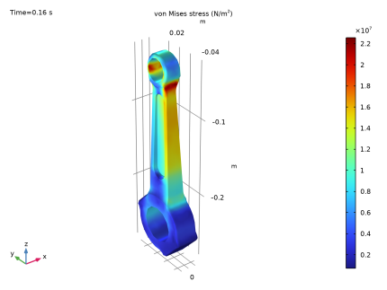
In the Settings window for Surface, click Replace Expression in the upper-right corner of the Expression section. From the menu, choose Multibody Analysis (comp2) > Multibody Dynamics > Stress > mbd.misesGp - von Mises stress - N/m².
|
|
1
|
|
2
|
|
3
|
Clear the Plot dataset edges checkbox.
|
|
4
|
|
5
|
|
1
|
|
2
|
|
3
|
Locate the Data section. From the Dataset list, choose Study: Multibody Analysis/Solution 2 (3) (sol2).
|
|
1
|
|
2
|
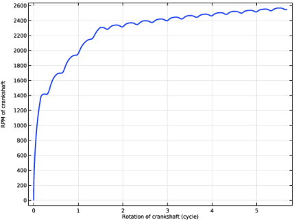
In the Settings window for Global, click Replace Expression in the upper-right corner of the y-Axis Data section. From the menu, choose Multibody Analysis (comp2) > Definitions > Variables > N - RPM of crankshaft - rad/s.
|
|
3
|
|
4
|
|
5
|
|
6
|
|
7
|
|
1
|
|
2
|
|
3
|
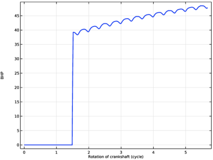
Select the x-axis label checkbox. In the associated text field, type Rotation of crankshaft (cycle).
|
|
4
|
|
5
|
|
1
|
|
2
|
|
3
|
|
1
|
|
2
|
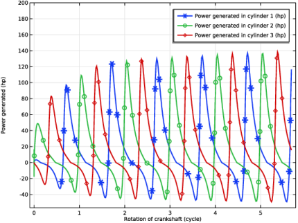
In the Settings window for Global, click Replace Expression in the upper-right corner of the y-Axis Data section. From the menu, choose Multibody Analysis (comp2) > Definitions > Variables > P1 - Power generated in cylinder 1 (hp) - 1.
|
|
3
|
Click Add Expression in the upper-right corner of the y-Axis Data section. From the menu, choose Multibody Analysis (comp2) > Definitions > Variables > P2 - Power generated in cylinder 2 (hp) - 1.
|
|
4
|
Click Add Expression in the upper-right corner of the y-Axis Data section. From the menu, choose Multibody Analysis (comp2) > Definitions > Variables > P3 - Power generated in cylinder 3 (hp) - 1.
|
|
5
|
Locate the Coloring and Style section. Find the Line markers subsection. From the Marker list, choose Cycle.
|
|
6
|
|
7
|
|
8
|
|
9
|
|
1
|
|
2
|
|
3
|
Select the Manual axis limits checkbox.
|
|
4
|
|
5
|
|
1
|
|
2
|
|
3
|
|
1
|
|
2
|
In the Settings window for Global, click Replace Expression in the upper-right corner of the y-Axis Data section. From the menu, choose Multibody Analysis (comp2) > Definitions > Variables > BHP - Brake horse power - rad.
|
|
3
|
|
1
|
|
2
|
|
3
|
|
1
|
|
2
|
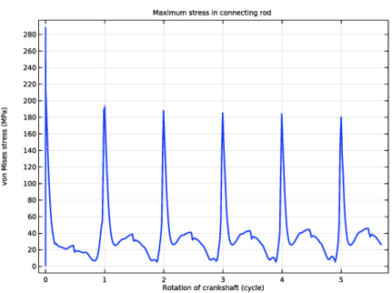
In the Settings window for Global, click Replace Expression in the upper-right corner of the y-Axis Data section. From the menu, choose Multibody Analysis (comp2) > Definitions > Variables > MaxStress_cr - Maximum stress in connecting rod - N/m².
|
|
3
|
Locate the y-Axis Data section. In the table, enter the following settings:
|
|
4
|
|
5
|
|
6
|
|
1
|
|
2
|
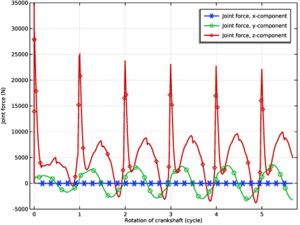
In the Settings window for 1D Plot Group, type Joint Force: Connecting Rod-Crank in the Label text field.
|
|
3
|
|
1
|
In the Model Builder window, expand the Joint Force: Connecting Rod-Crank node, then click Global 1.
|
|
2
|
In the Settings window for Global, click Replace Expression in the upper-right corner of the y-Axis Data section. From the menu, choose Multibody Analysis (comp2) > Multibody Dynamics > Hinge joints > Hinge Joint 2 > Joint force - N > mbd.hgj2.Fx - Joint force, x-component.
|
|
3
|
Click Add Expression in the upper-right corner of the y-Axis Data section. From the menu, choose Multibody Analysis (comp2) > Multibody Dynamics > Hinge joints > Hinge Joint 2 > Joint force - N > mbd.hgj2.Fy - Joint force, y-component.
|
|
4
|
Click Add Expression in the upper-right corner of the y-Axis Data section. From the menu, choose Multibody Analysis (comp2) > Multibody Dynamics > Hinge joints > Hinge Joint 2 > Joint force - N > mbd.hgj2.Fz - Joint force, z-component.
|
|
5
|
|
1
|
|
2
|
|
3
|
|
4
|
|
5
|
|
1
|
|
2
|
|
3
|
|
4
|