|
|
|
|
•
|
|
•
|
|
•
|
|
•
|
|
•
|
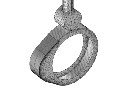
Change the discretization order of the dependent variable to Quadratic in order to increase the geometry shape order and improve the accuracy of the mesh normal used in the Cam–Follower connection node.
|
|
•
|
Use a fine mapped mesh, if possible, on a cam surface in order to improve the accuracy of the mesh normal used in the Cam–Follower connection node.
|
|
1
|
|
2
|
|
3
|
Click Add.
|
|
4
|
Click
|
|
5
|
|
6
|
Click
|
|
1
|
|
2
|
|
3
|
Click
|
|
4
|
Browse to the model’s Application Libraries folder and double-click the file radial_cam_follower_parameters.txt.
|
|
1
|
|
2
|
|
3
|
|
4
|
Click
|
|
5
|
Browse to the model’s Application Libraries folder and double-click the file radial_cam_follower.mphbin.
|
|
6
|
Click
|
|
1
|
|
2
|
|
3
|
|
4
|
Clear the Create pairs checkbox.
|
|
5
|
|
1
|
|
2
|
|
3
|
|
4
|
|
1
|
|
2
|
|
3
|
|
5
|
Select the Group by continuous tangent checkbox.
|
|
6
|
|
1
|
|
2
|
|
3
|
|
4
|
|
5
|
|
6
|
Click OK.
|
|
7
|
|
8
|
|
9
|
|
1
|
|
2
|
Go to the Add Material window.
|
|
3
|
|
4
|
Click the Add to Component button in the window toolbar.
|
|
5
|
|
1
|
|
2
|
|
1
|
|
2
|
|
1
|
|
2
|
|
3
|
|
4
|
|
5
|
|
6
|
Click OK.
|
|
7
|
|
8
|
|
9
|
|
1
|
|
2
|
|
3
|
|
4
|
|
5
|
|
6
|
|
1
|
|
2
|
|
3
|
Click
|
|
4
|
|
5
|
Click OK.
|
|
1
|
|
2
|
|
3
|
|
4
|
|
5
|
|
1
|
|
2
|
|
3
|
|
1
|
In the Model Builder window, under Component 1 (comp1) > Multibody Dynamics (mbd), Ctrl-click to select Rigid Material: Cam, Rigid Material: Follower, Rigid Material: Rocker Arm, Rigid Material: Valve, Rigid Material: Follower Guide, Rigid Material: Pin, and Rigid Material: Valve Guide.
|
|
2
|
Right-click and choose Group.
|
|
1
|
In the Model Builder window, under Component 1 (comp1) > Multibody Dynamics (mbd), Ctrl-click to select Hinge Joint 1 and Hinge Joint 2.
|
|
2
|
Right-click and choose Group.
|
|
1
|
In the Model Builder window, under Component 1 (comp1) > Multibody Dynamics (mbd), Ctrl-click to select Prismatic Joint 1 and Prismatic Joint 2.
|
|
2
|
Right-click and choose Group.
|
|
1
|
In the Model Builder window, under Component 1 (comp1) > Multibody Dynamics (mbd), Ctrl-click to select Slot Joint 1 and Slot Joint 2.
|
|
2
|
Right-click and choose Group.
|
|
1
|
|
2
|
|
3
|
|
1
|
|
2
|
|
3
|
Click the Custom button.
|
|
4
|
Locate the Element Size Parameters section.
|
|
5
|
|
6
|
|
7
|
Click
|
|
1
|
|
2
|
|
3
|
|
1
|
|
2
|
|
3
|
Click
|
|
4
|
|
5
|
Click OK.
|
|
6
|
|
7
|
|
1
|
|
2
|
|
3
|
|
4
|
Click
|
|
1
|
|
2
|
|
3
|
|
4
|
|
5
|
Click
|
|
1
|
|
2
|
|
3
|
In the Model Builder window, expand the Study 1 > Solver Configurations > Solution 1 (sol1) > Dependent Variables 1 node, then click Connection Force (comp1.mbd.cfc1.F).
|
|
4
|
|
5
|
|
6
|
In the Model Builder window, under Study 1 > Solver Configurations > Solution 1 (sol1) > Dependent Variables 1 click Reaction Moment (comp1.mbd.hgj1.pm1.RM).
|
|
7
|
|
8
|
|
9
|
|
1
|
|
2
|
|
3
|
|
4
|
|
5
|
|
1
|
|
2
|
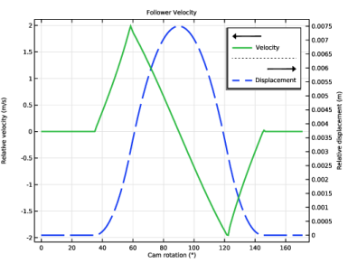
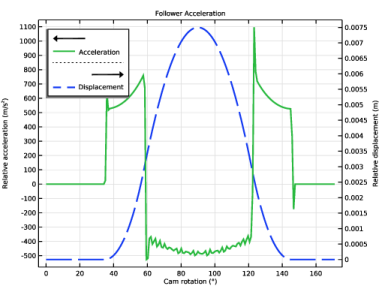
In the Settings window for Global, click Replace Expression in the upper-right corner of the y-Axis Data section. From the menu, choose Component 1 (comp1) > Multibody Dynamics > Prismatic joints > Prismatic Joint 1 > mbd.prj1.u - Relative displacement - m.
|
|
3
|
|
4
|
|
5
|
Click Replace Expression in the upper-right corner of the x-Axis Data section. From the menu, choose Component 1 (comp1) > Multibody Dynamics > Hinge joints > Hinge Joint 1 > mbd.hgj1.th - Relative rotation - rad.
|
|
6
|
|
7
|
|
8
|
Click to expand the Coloring and Style section. Find the Line style subsection. From the Line list, choose Dashed.
|
|
9
|
|
10
|
|
1
|
|
2
|
In the Settings window for Global, click Replace Expression in the upper-right corner of the y-Axis Data section. From the menu, choose Component 1 (comp1) > Multibody Dynamics > Prismatic joints > Prismatic Joint 1 > mbd.prj1.u_t - Relative velocity - m/s.
|
|
3
|
|
4
|
Locate the Coloring and Style section. Find the Line style subsection. From the Line list, choose Solid.
|
|
5
|
Locate the Legends section. In the table, enter the following settings:
|
|
6
|
|
7
|
|
1
|
|
2
|
|
3
|
|
1
|
|
2
|
In the Settings window for Global, click Replace Expression in the upper-right corner of the y-Axis Data section. From the menu, choose Component 1 (comp1) > Multibody Dynamics > Prismatic joints > Prismatic Joint 1 > mbd.prj1.u_tt - Relative acceleration - m/s².
|
|
3
|
Locate the Legends section. In the table, enter the following settings:
|
|
4
|
|
5
|
|
1
|
|
2
|
|
3
|
|
4
|
|
5
|
|
6
|
|
1
|
|
2
|
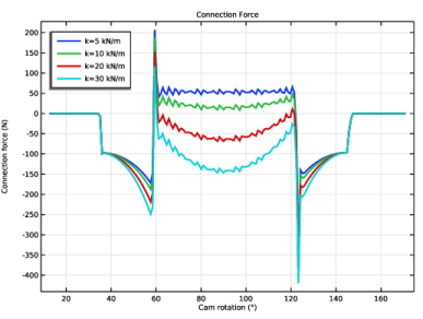
In the Settings window for Global, click Replace Expression in the upper-right corner of the y-Axis Data section. From the menu, choose Component 1 (comp1) > Multibody Dynamics > Cam–followers > Cam–Follower 1 > mbd.cfc1.F - Connection force - N.
|
|
3
|
|
4
|
Click Replace Expression in the upper-right corner of the x-Axis Data section. From the menu, choose Component 1 (comp1) > Multibody Dynamics > Hinge joints > Hinge Joint 1 > mbd.hgj1.th - Relative rotation - rad.
|
|
5
|
|
6
|
|
7
|
|
8
|
|
9
|
|
10
|
|
1
|
|
2
|
|
3
|
|
1
|
|
2
|
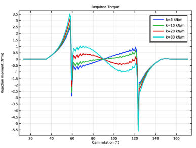
In the Settings window for Global, click Replace Expression in the upper-right corner of the y-Axis Data section. From the menu, choose Component 1 (comp1) > Multibody Dynamics > Hinge joints > Hinge Joint 1 > mbd.hgj1.pm1.RM - Reaction moment - N·m.
|
|
3
|
|
4
|
|
1
|
|
2
|
|
3
|