
|
|
|
|
1
|
|
2
|
|
3
|
Click Add.
|
|
4
|
|
5
|
Click Add.
|
|
6
|
Click
|
|
7
|
|
8
|
Click
|
|
1
|
|
2
|
|
1
|
|
2
|
|
3
|
|
4
|
|
1
|
|
2
|
|
3
|
|
4
|
In the x text field, type -0.35 -0.35 -0.35 -0.15 -0.15 -0.05 -0.05 -0.05 -0.05 0 0 0 0 -0.15+0.1*(sqrt(5)-2) -0.15+0.1*(sqrt(5)-2) -0.25 -0.25 -0.25.
|
|
5
|
In the y text field, type 0 0.3 0.3 0.4 0.4 0.4 0.4 1 1 1 1 0.3 0.3 0.3 0.3 0.3-0.05*(sqrt(5)-1) 0.3-0.05*(sqrt(5)-1) 0.
|
|
1
|
|
2
|
|
3
|
|
4
|
|
5
|
In the y text field, type 0.8 1.3+0.1*sqrt(2) 1.3+0.1*sqrt(2) 1.4+0.1*sqrt(2) 1.4+0.1*sqrt(2) 1.8 1.8 1.8 1.8 1.4 1.4 1.4 1.4 0.8.
|
|
6
|
Click
|
|
7
|
|
1
|
|
2
|
Select the object pol1 only.
|
|
1
|
|
2
|
Select the object c1 only.
|
|
3
|
|
4
|
|
5
|
Select the object copy1 only.
|
|
1
|
|
2
|
Click in the Graphics window and then press Ctrl+A to select all objects.
|
|
3
|
|
4
|
Select the Keep input objects checkbox.
|
|
1
|
|
2
|
|
3
|
|
4
|
Clear the Keep interior boundaries checkbox.
|
|
1
|
|
2
|
|
3
|
|
4
|
Clear the Keep interior boundaries checkbox.
|
|
1
|
|
2
|
|
1
|
|
2
|
|
3
|
|
4
|
Click
|
|
5
|
|
6
|
|
1
|
|
2
|
Go to the Add Material window.
|
|
3
|
|
4
|
Click the Add to Component button in the window toolbar.
|
|
5
|
|
1
|
|
2
|
|
1
|
In the Model Builder window, under Component 1 (comp1) > Multibody Dynamics (mbd) click Initial Values 1.
|
|
2
|
|
3
|
From the list, choose Locally defined.
|
|
4
|
Specify the du/dt vector as
|
|
1
|
|
3
|
|
4
|
From the list, choose Flexible.
|
|
1
|
|
3
|
|
4
|
From the list, choose Flexible.
|
|
1
|
|
2
|
|
3
|
|
4
|
|
5
|
|
1
|
|
2
|
|
3
|
|
4
|
|
1
|
|
3
|
|
4
|
|
5
|
From the list, choose Diagonal.
|
|
6
|
Specify the m matrix as
|
|
1
|
|
3
|
|
4
|
|
5
|
From the list, choose Diagonal.
|
|
6
|
|
7
|
Click to expand the Viscous Damping section. From the Damping type list, choose Total damping constant.
|
|
8
|
From the list, choose Diagonal.
|
|
9
|
|
1
|
|
2
|
|
3
|
|
1
|
|
2
|
|
1
|
|
2
|
|
3
|
|
1
|
|
2
|
|
3
|
Click
|
|
4
|
|
5
|
Click OK.
|
|
6
|
|
7
|
|
8
|
|
1
|
|
2
|
|
3
|
|
4
|
Click
|
|
1
|
|
2
|
|
3
|
|
4
|
|
1
|
|
2
|
|
3
|
|
4
|
|
1
|
|
2
|
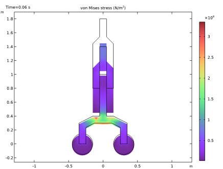
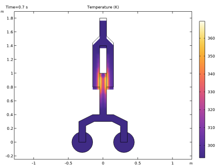
In the Settings window for Surface, click Replace Expression in the upper-right corner of the Expression section. From the menu, choose Component 1 (comp1) > Multibody Dynamics > Stress > mbd.misesGp - von Mises stress - N/m².
|
|
3
|
|
4
|
|
5
|
|
6
|
|
1
|
|
2
|
|
3
|
|
4
|
|
1
|
|
2
|
|
3
|
|
4
|
|
1
|
|
2
|
|
3
|
|
1
|
|
2
|
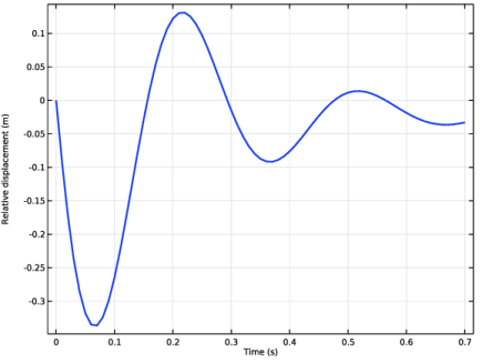
In the Settings window for Global, click Replace Expression in the upper-right corner of the y-Axis Data section. From the menu, choose Component 1 (comp1) > Multibody Dynamics > Prismatic joints > Prismatic Joint 1 > mbd.prj1.u - Relative displacement - m.
|
|
3
|
|
4
|
|
5
|
|
1
|
|
2
|
|
1
|
|
2
|
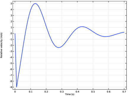
In the Settings window for Global, click Replace Expression in the upper-right corner of the y-Axis Data section. From the menu, choose Component 1 (comp1) > Multibody Dynamics > Prismatic joints > Prismatic Joint 1 > mbd.prj1.u_t - Relative velocity - m/s.
|
|
3
|
|
1
|
|
2
|
|
1
|
|
2
|
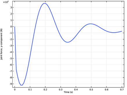
In the Settings window for Global, click Replace Expression in the upper-right corner of the y-Axis Data section. From the menu, choose Component 1 (comp1) > Multibody Dynamics > Prismatic joints > Prismatic Joint 1 > Joint force - N > mbd.prj1.Fy - Joint force, y-component.
|
|
3
|
|
1
|
|
2
|
|
3
|
|
1
|
|
2
|
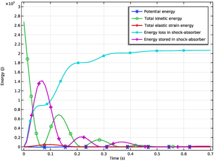
In the Settings window for Global, click Replace Expression in the upper-right corner of the y-Axis Data section. From the menu, choose Component 1 (comp1) > Definitions > Variables > Wp - Potential energy - J.
|
|
3
|
Click Add Expression in the upper-right corner of the y-Axis Data section. From the menu, choose Component 1 (comp1) > Multibody Dynamics > Global > mbd.Wk_tot - Total kinetic energy - J.
|
|
4
|
Click Add Expression in the upper-right corner of the y-Axis Data section. From the menu, choose Component 1 (comp1) > Multibody Dynamics > Global > mbd.Ws_tot - Total elastic strain energy - J.
|
|
5
|
Click Add Expression in the upper-right corner of the y-Axis Data section. From the menu, choose Component 1 (comp1) > Definitions > Variables > h_sa - Energy loss in shock-absorber - J.
|
|
6
|
Click Add Expression in the upper-right corner of the y-Axis Data section. From the menu, choose Component 1 (comp1) > Definitions > Variables > Ws_sa - Energy stored in shock-absorber - J.
|
|
7
|
|
8
|
|
9
|
|
10
|
|
1
|
|
2
|
|
3
|
|
4
|
|
5
|
|
6
|
|
1
|
|
2
|
|
3
|
|
4
|
|
1
|
|
2
|
|
3
|
|
4
|
|
5
|