PDF

Dynamics of a Hopping Hoop
Introduction
In this conceptual example, a hopping hoop is modeled using the Multibody Dynamics interface. The model setup is based on a problem described in Ref. 1 with slight modifications. The original problem discusses the dynamics of an ideal, massless, rigid ring with a point mass attached to its perimeter. In this example, the different types of motion are investigated, which a thin rolling ring-point mass system can exhibit. It is shown, that under certain conditions, the rolling ring can disconnect from the ground and lift into the air.
Model Definition
As shown in Figure 1, the 2D model geometry consists of a thin ring placed at one end of a fixed, flat surface.
Figure 1: Geometry of the ring with a point mass at the top, placed on a rectangular block.
Both the ring and the plane are modeled as rigid bodies. A point mass is attached to the top point of the ring. Unlike the original problem, where the ring is considered as massless, a small fraction of the ring’s total mass is uniformly distributed along its perimeter. The mass ratio of the system is γ. Thus, if m is the total mass of the system, a mass γm is assigned to the point mass and the remaining mass, (1 − γ)m, is assigned to the ring. Using the special case γ = 1, the configuration of the original problem can be recovered. Gravity is acting in the vertical direction.
The physical parameters used in the model are listed in Table 1. The fundamental model parameters are set to unity, as the exact numerical values are irrelevant for the general dynamics of the system.
Rc
0.75
The contact between the rolling ring and the plane is modeled using the Rigid Body Contact node, and frictional forces are included with the Friction subnode. The coefficient of friction between the ring and the plane is set to μ = 1.
The motion starts with the ring being in an unstable equilibrium, where the point mass is at the top of the ring. To nudge the ring into a rolling motion, initial linear and angular velocities are applied. A time-dependent study is run for different initial velocities.
Results and Discussion
When the ring is pushed forward with an initial velocity, it begins to roll. The mass at the top of the ring moves toward the ground plane accelerated by gravity. The translational velocity of the system along the plane increases. With the continued rotation of the ring, the point mass reaches the bottom most position and then moves up. While the point mass moves upward, the ring’s translational and rotational velocity decreases. When the point mass reaches top again, the ring velocity is at a minimum. Thus, during the revolution of the ring, the rotational speed of the system varies substantially.
Figure 2 shows the velocity of the ring for four different initial velocities. The cycloid path of the point mass and the center of gravity of the system are also plotted. For different initial velocities, the system exhibits different types of motions. For a small initial velocity (v0 = 0.1 m/s), the ring exhibits a pure rolling motion without any slipping or hopping. For a slightly increased initial velocity (v0 = 2.8 m/s), the ring rolls on the plane with some slipping. As the initial velocity is increased further (v0 = 3.1 m/s and v0 = 3.5 m/s), the ring initially rolls and then starts to hop. This is illustrated in Figure 2, where the trace of the center of gravity is colored red when the hoop is airborne. This part of the curve forms a projectile motion parabola.
Figure 2: Velocity of the ring at t = 5.2 s for four different initial velocities. The path of the point mass and center of gravity are also shown. The arrows proportional to contact forces.
Below, we look at some key features of the system for the different types of motions.
Pure Rolling
For a small initial velocity, the ring-mass system undergoes pure rolling without slipping or hopping. Figure 3 plots the variation of translational velocity of the ring center and the normalized angular velocity for two different initial velocities. As evident from the plot, the translational velocity of the center is equal to the angular velocity of the system for pure rolling. As the initial velocity increases, the velocity of the system increases.
Figure 3: Velocity as a function of rotation angle for v0 = 0.1 m/s and 2 m/s.
Figure 4: Energy as a function of rotation angle for v0 = 0.1 m/s.
In the case of pure rolling, the potential and kinetic energies of the system vary harmonically as shown in Figure 4. As the ring does not hop for low of initial velocities, the height of the center of mass of the ring does not change. Hence, the vertical position of the point mass is the only contributing factor for the harmonic variation of the energies.
The variations of normal and frictional contact forces are plotted in Figure 5. The motion of the system is driven by the horizontal force from friction, which causes the system to accelerate or decelerate. When the ring is in contact with the surface, the vertical contact force would be positive. When contact is lost, the normal contact force becomes zero. You can also see that as the initial velocity increases, the minimum contact force decreases.
Another condition for pure rolling is that the friction force cannot exceed the normal force. The ratio of friction force to normal force, also called friction force utilization factor, is plotted in Figure 6. The figure shows that for v0 = 0.1 m/s, only 38% of the available friction is utilized in the pure rolling case. This can also be interpreted as the minimum friction coefficient needed to maintain pure rolling. As the initial velocity increases, the friction force utilization factor also increases reaching a maximum value of 1, thus utilizing a larger fraction of the available friction force.
Figure 5: Contact and friction forces as a function of rotation angle for v0 = 0.1 m/s and m/s.
Figure 6: Friction utilization factor as a function of rotation angle for v0 = 0.1 m/s and 2 m/s.
Rolling with slipping
As the initial velocity is increased further, the ring starts to slip. The translational and angular velocities for v0 = 2.8 m/s are plotted in Figure 7. As shown in figure, the translational and angular velocities are no longer identical for this case. This is also evident from the friction utilization factor shown in Figure 10, which levels out at 1. As shown in Figure 7, the peak velocity is decreasing with each cycle. This system could reach a pure rolling state, when enough energy has dissipated. The system energy as a function of rotation angle is plotted in Figure 8 (note that the total energy in this plot is defined as the sum of potential and kinetic energies).
Figure 7: Velocity as a function of rotation angle for v0 = 2.8 m/s.
Figure 8: Energy as a function of rotation angle for v0 = 2.8 m/s.
Figure 9: Contact and friction forces as a function of rotation angle for v0 = 2.8 m/s.
Figure 10: Friction utilization factor as a function of rotation angle for v0 = 2.8 m/s.
Rolling with Hopping
For the initial velocity of v0 = 3.1 m/s, the ring hops just before completing one revolution. The plot of translational and angular velocity (Figure 11) shows that the angular velocity is constant when the hoop is airborne. The system energy as a function of rotation angle is plotted in Figure 12. Between 350° and 390°, the potential energy of the system is larger than zero, causing the kinetic energy to be larger than the total energy. This is one consequence of the upward motion of the ring’s center.
Figure 11: Velocity as a function of rotation angle for v0 = 3.1 m/s.
Figure 12: Energy as a function of rotation angle for v0 = 3.1 m/s.
Figure 13: Contact and friction forces as a function of rotation angle for v0 = 3.1 m/s.
Figure 14: Friction utilization factor as a function of rotation angle for v0 = 3.1 m/s.
Reference
1. J.E. Littlewood, A Mathematician’s Miscellany, MR 087285, Methuen, London, 1953.
Application Library path: Multibody_Dynamics_Module/Verification_Examples/hopping_hoop
Modeling Instructions
From the File menu, choose New.
New
In the New window, click  Model Wizard.
Model Wizard
1
In the Model Wizard window, click  2D.
2
In the Select Physics tree, select Structural Mechanics > Multibody Dynamics (mbd).
3
Click Add.
4
Click  Study.
5
In the Select Study tree, select General Studies > Time Dependent.
6
Global Definitions
Parameters 1
1
In the Model Builder window, under Global Definitions click Parameters 1.
2
In the Settings window for Parameters, locate the Parameters section.
3
Click  Load from File.
4
Geometry 1
Circle 1 (c1)
1
In the Geometry toolbar, click  Circle.
2
In the Settings window for Circle, locate the Size and Shape section.
3
In the Radius text field, type Rc.
4
Click to expand the Layers section. In the table, enter the following settings:
5
Click  Build Selected.
Delete Entities 1 (del1)
1
In the Model Builder window, right-click Geometry 1 and choose Delete Entities.
2
In the Settings window for Delete Entities, locate the Entities or Objects to Delete section.
3
From the Geometric entity level list, choose Domain.
4
On the object c1, select Domain 5 only.
5
Click  Build Selected.
Rectangle 1 (r1)
1
In the Geometry toolbar, click  Rectangle.
2
In the Settings window for Rectangle, locate the Size and Shape section.
3
In the Width text field, type Lbase.
4
In the Height text field, type 0.1.
5
Locate the Position section. In the x text field, type -0.1.
6
In the y text field, type -1.1.
7
Click  Build Selected.
Form Union (fin)
1
In the Model Builder window, under Component 1 (comp1) > Geometry 1 click Form Union (fin).
2
In the Settings window for Form Union/Assembly, locate the Form Union/Assembly section.
3
From the Action list, choose Form an assembly.
4
Clear the Create pairs checkbox.
5
Click  Build Selected.
Definitions
Point Mass
1
In the Definitions toolbar, click  Explicit.
2
In the Settings window for Explicit, type Point Mass in the Label text field.
3
Locate the Input Entities section. From the Geometric entity level list, choose Point.
4
Ring Edges
1
In the Definitions toolbar, click  Explicit.
2
In the Settings window for Explicit, type Ring Edges in the Label text field.
3
Locate the Input Entities section. From the Geometric entity level list, choose Boundary.
4
5
Select the Group by continuous tangent checkbox.
Average: Point Mass
1
In the Definitions toolbar, click  Nonlocal Couplings and choose Average.
2
In the Settings window for Average, type Average: Point Mass in the Label text field.
3
Locate the Source Selection section. From the Geometric entity level list, choose Point.
4
From the Selection list, choose Point Mass.
Average: Ring Edges
1
Right-click Average: Point Mass and choose Duplicate.
2
In the Settings window for Average, type Average: Ring Edges in the Label text field.
3
Locate the Source Selection section. From the Geometric entity level list, choose Boundary.
4
From the Selection list, choose Ring Edges.
Variables 1
1
In the Model Builder window, right-click Definitions and choose Variables.
2
In the Settings window for Variables, locate the Variables section.
3
Multibody Dynamics (mbd)
1
In the Model Builder window, under Component 1 (comp1) click Multibody Dynamics (mbd).
2
In the Settings window for Multibody Dynamics, click to expand the Initial Values section.
3
Specify the du/dt vector as
4
5
In the dϕ/dt text field, type -omega0.
Rigid Material: Plane
1
In the Physics toolbar, click  Domains and choose Rigid Material.
2
In the Settings window for Rigid Material, type Rigid Material: Plane in the Label text field.
3
4
Locate the Density section. From the ρ list, choose User defined.
Fixed Constraint 1
In the Physics toolbar, click  Attributes and choose Fixed Constraint.
Rigid Material: Ring
1
In the Physics toolbar, click  Domains and choose Rigid Material.
2
In the Settings window for Rigid Material, type Rigid Material: Ring in the Label text field.
3
4
Locate the Density section. From the ρ list, choose User defined.
Mass and Moment of Inertia 1
1
In the Physics toolbar, click  Attributes and choose Mass and Moment of Inertia.
2
In the Settings window for Mass and Moment of Inertia, locate the Center of Mass section.
3
From the list, choose Centroid of selected entities.
4
From the Entity level list, choose Point.
5
Locate the Mass and Moment of Inertia section. In the m text field, type mtot*gamma.
Center of Mass: Point 1
1
In the Model Builder window, click Center of Mass: Point 1.
2
In the Settings window for Center of Mass: Point, locate the Point Selection section.
3
From the Selection list, choose Point Mass.
Added Mass: Ring
1
In the Physics toolbar, click  Boundaries and choose Added Mass.
2
In the Settings window for Added Mass, type Added Mass: Ring in the Label text field.
3
Locate the Boundary Selection section. From the Selection list, choose Ring Edges.
4
Locate the Added Mass section. From the Mass type list, choose Total mass.
5
In the m text field, type mtot*(1-gamma).
Gravity 1
In the Physics toolbar, click  Global and choose Gravity.
Rigid Body Contact 1
1
In the Physics toolbar, click  Global and choose Rigid Body Contact.
2
In the Settings window for Rigid Body Contact, locate the Source section.
3
From the Source list, choose Rigid Material: Ring.
4
Locate the Destination section. From the Shape list, choose Planar.
5
Locate the Boundary Selection, Destination section. Click to select the  Activate Selection toggle button.
6
7
Locate the Contact Settings section. In the fp text field, type 0.001.
8
In the τn text field, type 0.05[ms].
9
Select the Compute viscous contact dissipation checkbox.
Friction 1
1
In the Physics toolbar, click  Attributes and choose Friction.
2
In the Settings window for Friction, locate the Friction section.
3
In the μ text field, type mu.
4
In the v0 text field, type 1e-4.
5
Click to expand the Advanced section. Select the Compute frictional dissipation checkbox.
Mesh 1
Edge 1
1
In the Mesh toolbar, click  More Generators and choose Edge.
2
In the Settings window for Edge, locate the Boundary Selection section.
3
From the Selection list, choose Ring Edges.
Distribution 1
1
Right-click Edge 1 and choose Distribution.
2
In the Settings window for Distribution, locate the Distribution section.
3
In the Number of elements text field, type 10.
Mapped 1
In the Mesh toolbar, click  Mapped.
Distribution 1
1
Right-click Mapped 1 and choose Distribution.
2
3
In the Settings window for Distribution, locate the Distribution section.
4
In the Number of elements text field, type 1.
5
Click  Build All.
Study 1
Parametric Sweep
1
In the Study toolbar, click  Parametric Sweep.
2
In the Settings window for Parametric Sweep, locate the Study Settings section.
3
4
Step 1: Time Dependent
1
In the Model Builder window, click Step 1: Time Dependent.
2
In the Settings window for Time Dependent, locate the Study Settings section.
3
In the Output times text field, type range(0,dt,t_end).
4
From the Tolerance list, choose User controlled.
5
In the Relative tolerance text field, type 0.0001.
Solution 1 (sol1)
1
In the Study toolbar, click  Show Default Solver.
2
In the Model Builder window, expand the Solution 1 (sol1) node, then click Time-Dependent Solver 1.
3
In the Settings window for Time-Dependent Solver, click to expand the Time Stepping section.
4
From the Maximum BDF order list, choose 3.
5
Find the Algebraic variable settings subsection. From the Consistent initialization list, choose Off.
6
In the Study toolbar, click  Compute.
Follow the instructions below to plot the velocity of the ring and the path of the point mass and center of gravity as shown in Figure 2.
Results
Velocity (mbd)
1
In the Model Builder window, under Results click Velocity (mbd).
2
In the Settings window for 2D Plot Group, click to expand the Title section.
3
From the Title type list, choose None.
4
Locate the Color Legend section. Clear the Show legends checkbox.
Domain Numbers
1
In the Model Builder window, expand the Velocity (mbd) node, then click Domain Numbers.
2
In the Settings window for Surface, locate the Expression section.
3
In the Expression text field, type mbd.vel.
4
Locate the Coloring and Style section. From the Color table list, choose SpectrumLight.
Arrow Line
In the Model Builder window, right-click Arrow Line and choose Delete.
Velocity (mbd)
In the Model Builder window, under Results click Velocity (mbd).
Point Trajectories: Point Mass
1
In the Velocity (mbd) toolbar, click  More Plots and choose Point Trajectories.
2
In the Settings window for Point Trajectories, type Point Trajectories: Point Mass in the Label text field.
3
Locate the Selection section. From the Selection list, choose Point Mass.
4
Locate the Coloring and Style section. Find the Line style subsection. From the Type list, choose Tube.
5
Select the Radius scale factor checkbox. In the associated text field, type 0.03.
6
Find the Point style subsection. From the Type list, choose Point.
7
In the Point radius expression text field, type 0.15.
8
Select the Radius scale factor checkbox.
9
From the Color list, choose Magenta.
Point Trajectories: Center of Gravity
1
Right-click Point Trajectories: Point Mass and choose Duplicate.
2
In the Settings window for Point Trajectories, type Point Trajectories: Center of Gravity in the Label text field.
3
Locate the Trajectory Data section. From the Plot data list, choose Global.
4
In the X-expression text field, type aveop1(x)*gamma+aveop2(x)*(1-gamma).
5
In the Y-expression text field, type aveop1(y)*gamma+aveop2(y)*(1-gamma).
6
Locate the Coloring and Style section. Find the Point style subsection. From the Type list, choose None.
Color Expression 1
1
Right-click Point Trajectories: Center of Gravity and choose Color Expression.
2
In the Settings window for Color Expression, locate the Expression section.
3
In the Expression text field, type aveop2(y)>1e-3.
4
Locate the Coloring and Style section. From the Color table list, choose TrafficLight.
Point Trajectories: Contact Force
1
In the Model Builder window, right-click Point Trajectories: Point Mass and choose Duplicate.
2
In the Settings window for Point Trajectories, type Point Trajectories: Contact Force in the Label text field.
3
Locate the Trajectory Data section. From the Plot data list, choose Global.
4
In the X-expression text field, type aveop2(x).
5
In the Y-expression text field, type aveop2(y)-Rc.
6
Locate the Coloring and Style section. Find the Line style subsection. From the Type list, choose None.
7
Find the Point style subsection. From the Type list, choose Arrow.
8
In the Arrow, Y-component text field, type -mbd.rbc1.Fny.
9
Select the Scale factor checkbox. In the associated text field, type 0.08.
10
From the Color list, choose Red.
Point Trajectories: Friction Force
1
Right-click Point Trajectories: Contact Force and choose Duplicate.
2
In the Settings window for Point Trajectories, type Point Trajectories: Friction Force in the Label text field.
3
Locate the Coloring and Style section. Find the Point style subsection. In the Arrow, X-component text field, type mbd.rbc1.Ffx.
4
In the Arrow, Y-component text field, type 0.
5
Click to expand the Inherit Style section. From the Plot list, choose Point Trajectories: Contact Force.
Similarly loop through the different initial velocities to reproduce the plots in Figure 2.
Follow the instructions below to see the dynamics of the system in 3D.
Extrusion 2D 1
1
In the Results toolbar, click  More Datasets and choose Extrusion 2D.
2
In the Settings window for Extrusion 2D, locate the Data section.
3
From the Dataset list, choose Study 1/Parametric Solutions 1 (sol2).
4
Locate the Extrusion section. Find the Embedding subsection. From the Map plane to list, choose xz-plane.
Velocity (3D)
1
In the Results toolbar, click  3D Plot Group.
2
In the Settings window for 3D Plot Group, type Velocity (3D) in the Label text field.
3
Locate the Data section. From the Parameter value (v0 (m/s)) list, choose 3.1.
4
Locate the Plot Settings section. From the Frame list, choose Spatial  (x, y, z).
5
Locate the Color Legend section. Clear the Show legends checkbox.
Volume 1
1
Right-click Velocity (3D) and choose Volume.
2
In the Settings window for Volume, locate the Expression section.
3
In the Expression text field, type mbd.vel.
4
Locate the Coloring and Style section. From the Color table list, choose SpectrumLight.
Deformation 1
1
Right-click Volume 1 and choose Deformation.
2
In the Settings window for Deformation, locate the Expression section.
3
In the y-component text field, type 0.
4
In the z-component text field, type v.
5
Locate the Scale section.
6
Select the Scale factor checkbox. In the associated text field, type 1.
Velocity (3D)
In the Model Builder window, under Results click Velocity (3D).
Point Trajectories 1
1
In the Velocity (3D) toolbar, click  More Plots and choose Point Trajectories.
2
In the Settings window for Point Trajectories, locate the Trajectory Data section.
3
From the Plot data list, choose Global.
4
In the x-expression text field, type aveop1(x).
5
In the z-expression text field, type aveop1(y).
6
Locate the Coloring and Style section. Find the Line style subsection. From the Type list, choose Tube.
Color Expression 1
1
Right-click Point Trajectories 1 and choose Color Expression.
2
In the Settings window for Color Expression, locate the Expression section.
3
In the Expression text field, type aveop2(y)>1e-3.
4
Locate the Coloring and Style section. From the Color table list, choose TrafficLight.
Velocity (3D)
1
In the Model Builder window, under Results click Velocity (3D).
2
In the Velocity (3D) toolbar, click  Plot.
Follow the instructions below to plot translational and normalized angular velocities as a function of rotation angle for v0 = 0.1 m/s as shown in Figure 3.
Velocity vs. Rotation Angle
1
In the Results toolbar, click  1D Plot Group.
2
In the Settings window for 1D Plot Group, type Velocity vs. Rotation Angle in the Label text field.
3
Locate the Data section. From the Dataset list, choose Study 1/Parametric Solutions 1 (sol2).
4
Click to expand the Title section. From the Title type list, choose None.
5
Locate the Data section. From the Parameter selection (v0) list, choose From list.
6
In the Parameter values (v0 (m/s)) list, choose 0.1 and 2.
7
Locate the Plot Settings section.
8
Select the x-axis label checkbox. In the associated text field, type Rotation Angle (°).
9
Select the y-axis label checkbox. In the associated text field, type Velocity (m/s).
10
Locate the Axis section. Select the Manual axis limits checkbox.
11
In the x minimum text field, type 0.
12
In the x maximum text field, type 1080.
13
In the y minimum text field, type -0.1.
14
In the y maximum text field, type 14.
15
Locate the Grid section. Select the Manual spacing checkbox.
16
In the x spacing text field, type 180.
17
Locate the Legend section. In the Maximum relative width text field, type 1.
Global 1
1
Right-click Velocity vs. Rotation Angle and choose Global.
2
In the Settings window for Global, locate the y-Axis Data section.
3
4
Locate the x-Axis Data section. From the Axis source data list, choose Inner solutions.
5
From the Parameter list, choose Expression.
6
In the Expression text field, type -mbd.rd2.thz.
7
From the Unit list, choose °.
8
Click to expand the Coloring and Style section. Find the Line style subsection. From the Line list, choose Cycle.
9
From the Width list, choose 4.
10
In the Velocity vs. Rotation Angle toolbar, click  Plot.
Follow the instructions below to plot translational and normalized angular velocities as a function of time.
Velocity vs. Time
1
In the Model Builder window, right-click Velocity vs. Rotation Angle and choose Duplicate.
2
In the Settings window for 1D Plot Group, type Velocity vs. Time in the Label text field.
3
Locate the Plot Settings section. In the x-axis label text field, type Time (s).
4
Locate the Data section. In the Parameter values (v0 (m/s)) list box, select 3.1.
5
Locate the Axis section. Clear the Manual axis limits checkbox.
6
Locate the Grid section. Clear the Manual spacing checkbox.
Global 1
1
In the Model Builder window, expand the Velocity vs. Time node, then click Global 1.
2
In the Settings window for Global, locate the x-Axis Data section.
3
From the Parameter list, choose Time.
4
In the Velocity vs. Time toolbar, click  Plot.
Follow the instructions below to plot energy as a function of rotation angle for v0 = 0.1 m/s as shown in Figure 4.
Energy vs. Rotation Angle
1
In the Model Builder window, right-click Velocity vs. Rotation Angle and choose Duplicate.
2
In the Settings window for 1D Plot Group, type Energy vs. Rotation Angle in the Label text field.
3
Locate the Data section. In the Parameter values (v0 (m/s)) list box, select 0.1.
4
Locate the Plot Settings section. In the y-axis label text field, type Energy (J).
5
Locate the Grid section. In the y spacing text field, type 5.
6
Locate the Axis section. In the y minimum text field, type -16.
7
In the y maximum text field, type 30.
Global 1
1
In the Model Builder window, expand the Energy vs. Rotation Angle node, then click Global 1.
2
In the Settings window for Global, locate the y-Axis Data section.
3
4
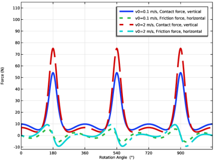
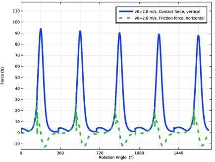
Click Add Expression in the upper-right corner of the y-Axis Data section. From the menu, choose Component 1 (comp1) > Multibody Dynamics > Rigid body contacts > Rigid Body Contact 1 > Friction > mbd.rbc1.Wf - Frictional energy dissipation - J.
5
Locate the Coloring and Style section. Find the Line style subsection. From the Line list, choose Solid.
6
In the Energy vs. Rotation Angle toolbar, click  Plot.
Follow the instructions below to plot energy as a function of time.
Energy vs. Time
1
In the Model Builder window, right-click Energy vs. Rotation Angle and choose Duplicate.
2
In the Settings window for 1D Plot Group, type Energy vs. Time in the Label text field.
3
Locate the Data section. In the Parameter values (v0 (m/s)) list box, select 3.1.
4
Locate the Plot Settings section. In the x-axis label text field, type Time (s).
5
Locate the Axis section. Clear the Manual axis limits checkbox.
6
Locate the Grid section. Clear the Manual spacing checkbox.
Global 1
1
In the Model Builder window, expand the Energy vs. Time node, then click Global 1.
2
In the Settings window for Global, locate the x-Axis Data section.
3
From the Parameter list, choose Time.
4
In the Energy vs. Time toolbar, click  Plot.
Follow the instructions below to plot contact and friction forces for v0 = 0.1 m/s as shown in Figure 5.
Contact Forces
1
In the Model Builder window, right-click Velocity vs. Rotation Angle and choose Duplicate.
2
In the Settings window for 1D Plot Group, type Contact Forces in the Label text field.
3
Locate the Plot Settings section. In the y-axis label text field, type Force (N).
4
Locate the Grid section. In the y spacing text field, type 10.
5
Locate the Axis section. In the y maximum text field, type 115.
6
In the y minimum text field, type -12.
Global 1
1
In the Model Builder window, expand the Contact Forces node, then click Global 1.
2
In the Settings window for Global, locate the y-Axis Data section.
3
Click  Clear Table.
4
5
In the Contact Forces toolbar, click  Plot.
Follow the instructions below to plot friction utilization factor for v0 = 0.1 m/s as shown in Figure 6.
Friction Utilization Factor
1
In the Model Builder window, right-click Contact Forces and choose Duplicate.
2
In the Settings window for 1D Plot Group, locate the Title section.
3
From the Title type list, choose Label.
4
In the Label text field, type Friction Utilization Factor.
5
Locate the Plot Settings section. Clear the y-axis label checkbox.
6
Locate the Grid section. In the y spacing text field, type 0.2.
7
Locate the Axis section. In the y maximum text field, type 1.6.
8
In the y minimum text field, type -1.1.
Global 1
1
In the Model Builder window, expand the Friction Utilization Factor node, then click Global 1.
2
In the Settings window for Global, locate the y-Axis Data section.
3
Click  Clear Table.
4
5
In the Friction Utilization Factor toolbar, click  Plot.
Follow the instructions below to plot velocity as a function of rotation angle for v0 = 2.8 m/s as shown in Figure 7.
Velocity vs. Rotation Angle
1
In the Model Builder window, under Results click Velocity vs. Rotation Angle.
2
In the Settings window for 1D Plot Group, locate the Data section.
3
In the Parameter values (v0 (m/s)) list box, select 2.8.
4
Locate the Axis section. In the x maximum text field, type 1740.
5
In the y maximum text field, type 13.
6
In the y minimum text field, type 2.
7
In the Velocity vs. Rotation Angle toolbar, click  Plot.
Follow the instructions below to plot energy as a function of rotation angle for v0 = 2.8 m/s as shown in Figure 8.
Energy vs. Rotation Angle
1
In the Model Builder window, click Energy vs. Rotation Angle.
2
In the Settings window for 1D Plot Group, locate the Data section.
3
In the Parameter values (v0 (m/s)) list box, select 2.8.
4
Locate the Axis section. In the x maximum text field, type 1740.
5
In the y maximum text field, type 47.
6
In the Energy vs. Rotation Angle toolbar, click  Plot.
Follow the instructions below to plot contact and friction forces for v0 = 2.8 m/s as shown in Figure 9.
Contact Forces
1
In the Model Builder window, click Contact Forces.
2
In the Settings window for 1D Plot Group, locate the Data section.
3
In the Parameter values (v0 (m/s)) list box, select 2.8.
4
Locate the Axis section. In the y maximum text field, type 118.
5
In the y minimum text field, type -15.
6
In the x maximum text field, type 1740.
7
In the Contact Forces toolbar, click  Plot.
Follow the instructions below to plot friction utilization factor for v0 = 2.8 m/s as shown in Figure 10.
Friction Utilization Factor
1
In the Model Builder window, click Friction Utilization Factor.
2
In the Settings window for 1D Plot Group, locate the Data section.
3
In the Parameter values (v0 (m/s)) list box, select 2.8.
4
Locate the Axis section. In the x maximum text field, type 1740.
5
In the Friction Utilization Factor toolbar, click  Plot.
Follow the instructions below to plot velocity as a function of rotation angle for v0 = 3.1 m/s as shown in Figure 11.
Velocity vs. Rotation Angle
1
In the Model Builder window, click Velocity vs. Rotation Angle.
2
In the Settings window for 1D Plot Group, locate the Data section.
3
In the Parameter values (v0 (m/s)) list box, select 3.1.
4
Locate the Axis section. In the x maximum text field, type 1440.
5
In the y minimum text field, type 1.
6
In the Velocity vs. Rotation Angle toolbar, click  Plot.
Follow the instructions below to plot energy as a function of rotation angle for v0 = 2.8 m/s as shown in Figure 12.
Energy vs. Rotation Angle
1
In the Model Builder window, click Energy vs. Rotation Angle.
2
In the Settings window for 1D Plot Group, locate the Data section.
3
In the Parameter values (v0 (m/s)) list box, select 3.1.
4
Locate the Axis section. In the x maximum text field, type 1440.
5
In the y maximum text field, type 46.
6
In the Energy vs. Rotation Angle toolbar, click  Plot.
Follow the instructions below to plot contact and friction forces for v0 = 3.1 m/s as shown in Figure 13.
Contact Forces
1
In the Model Builder window, click Contact Forces.
2
In the Settings window for 1D Plot Group, locate the Data section.
3
In the Parameter values (v0 (m/s)) list box, select 3.1.
4
Locate the Axis section. In the x maximum text field, type 1440.
5
In the y maximum text field, type 105.
6
In the Contact Forces toolbar, click  Plot.
Follow the instructions below to plot friction utilization factor for v0 = 3.1 m/s as shown in Figure 14.
Friction Utilization Factor
1
In the Model Builder window, click Friction Utilization Factor.
2
In the Settings window for 1D Plot Group, locate the Data section.
3
In the Parameter values (v0 (m/s)) list box, select 3.1.
4
Locate the Axis section. In the x maximum text field, type 1440.
5
In the Friction Utilization Factor toolbar, click  Plot.
Velocity (3D), Velocity (mbd), Velocity vs. Rotation Angle, Velocity vs. Time
1
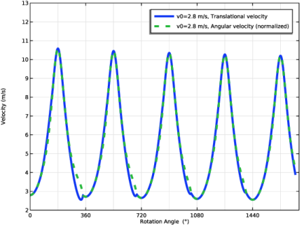
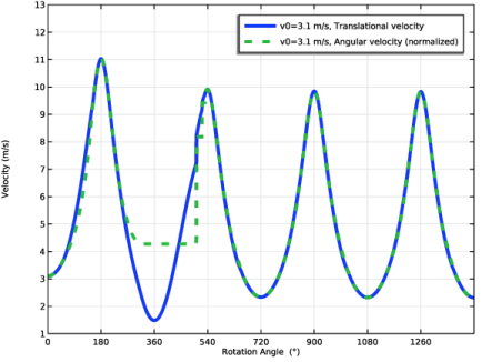
In the Model Builder window, under Results, Ctrl-click to select Velocity (mbd), Velocity (3D), Velocity vs. Rotation Angle, and Velocity vs. Time.
2
Velocity
In the Settings window for Group, type Velocity in the Label text field.
Energy vs. Rotation Angle, Energy vs. Time
1
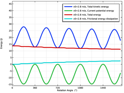
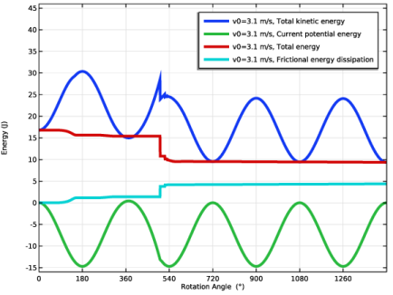
In the Model Builder window, under Results, Ctrl-click to select Energy vs. Rotation Angle and Energy vs. Time.
2
Energy
In the Settings window for Group, type Energy in the Label text field.
Contact Forces, Friction Utilization Factor
1
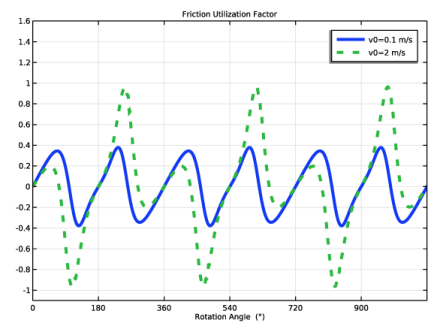
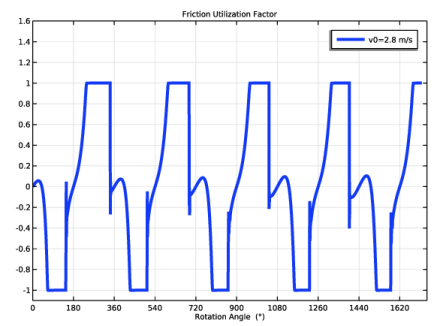
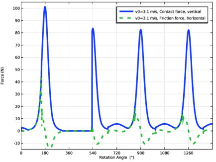
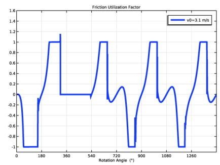
In the Model Builder window, under Results, Ctrl-click to select Contact Forces and Friction Utilization Factor.
2
Contact Forces
In the Settings window for Group, type Contact Forces in the Label text field.
Velocity
1
In the Results toolbar, click  Animation and choose Player.
2
In the Settings window for Animation, type Velocity in the Label text field.
3
Locate the Scene section. From the Subject list, choose Velocity (mbd).
4
Locate the Animation Editing section. From the Parameter value (v0 (m/s)) list, choose 3.1.
5
Locate the Frames section. In the Number of frames text field, type 100.
Velocity (3D)
1
Right-click Velocity and choose Duplicate.
2
In the Settings window for Animation, type Velocity (3D) in the Label text field.
3
Locate the Scene section. From the Subject list, choose Velocity (3D).